Interpretation of Neural Networks

By LI Haoyang 2020.11.18

Content

Generalization

Understanding deep learning requires rethinking generalization - ICLR 2017

Chiyuan Zhang, Samy Bengio, Moritz Hardt, Benjamin Recht, Oriol Vinyals. Understanding deep learning requires rethinking generalization. ICLR 2017. arXiv:1611.03530

Conventional wisdom attributes small generalization error either to properties of the model family, or to the regularization techniques used during training.

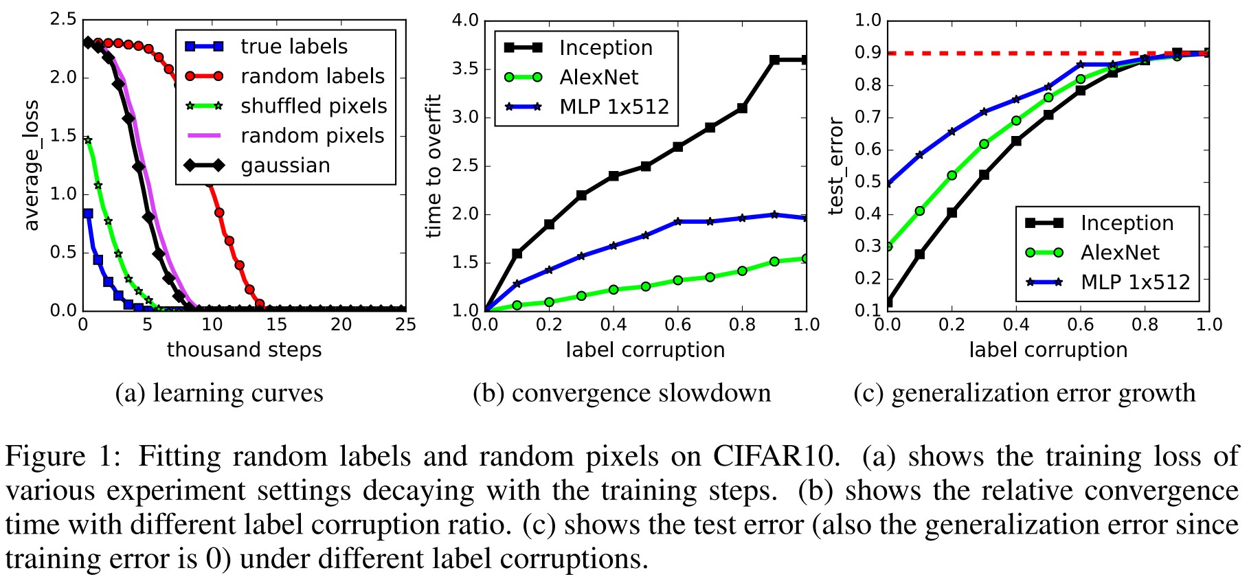
Specifically, our experiments establish that state-of-the-art convolutional networks for image classification trained with stochastic gradient methods easily fit a random labeling of the training data.

The CNN can learn nonsense (to human).

Discoveries

Their central finding is that

Deep neural networks easily fit random labels.

leading the following perspectives:

• The effective capacity of neural networks is sufficient for memorizing the entire data set.
• Even optimization on random labels remains easy.
• Randomizing labels is solely a data transformation, leaving all other properties of the learning problem unchanged.

We show that explicit forms of regularization, such as weight decay, dropout, and data augmentation, do not adequately explain the generalization error of neural networks.

Explicit regularization may improve generalization performance, but is neither necessary nor by itself sufficient for controlling generalization error.

We complement our empirical observations with a theoretical construction showing that generically large neural networks can express any labeling of the training data.

The neural network is very powerful and expressive.

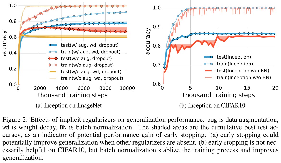
Since SGD is an implicit regularization (i.e. For linear models, SGD always converges to a solution with small norm.)

Though this doesn’t explain why certain architectures generalize better than other architectures, it does suggest that more investigation is needed to understand exactly what the properties are inherited by models that were trained using SGD.

Implications

Rademacher complexity and VC-dimension Rademacher complexity is commonly used and flexible complexity measure of a hypothesis class. The empirical Rademacher complexity of a hypothesis class $\mathcal{H}$ on a dataset $\{x_1,\dots,x_n\}$ is defined as

where $\sigma_i,\dots,\sigma_n\in\{-1,+1\}$ are i.i.d. uniform random variables.

It measures the ability of learning random labeled binary data for hypothesis space.

This definition closely resembles our randomization test.

Their randomization tests suggest that many neural networks fit the training set with random labels perfectly, implying that $\hat{\mathfrak{R}}_n(\mathcal{H})\approx 1$ for the corresponding model class $\mathcal{H}$.

Therefore, Rademacher complexity can not explain why some model (hypothesis space) is better in terms of generalization.

A similar reasoning applies to VC-dimension and its continuous analog fat-shattering dimension, unless we further restrict the network.

Uniform stability Uniform stability of an algorithm A measures how sensitive the algorithm is to the replacement of a single example. However, it is solely a property of the algorithm, which does not take into account specifics of the data or the distribution of the labels.

The role of regularization

They consider the following regularizers:

• Data augmentation: augment the training set via domain-specific transformations.
• Weight decay: equivalent to a $\ell_2$ regularizer on the weights; also equivalent to a hard constrain of the weights to an Euclidean ball, with the radius decided by the amount of weight decay.
• Dropout: mask out each element of a layer output randomly with a given dropout probability.
• Early stopping: stop the training process earlier.
• Batch Normalization: normalize the layer responses within each mini-batch.

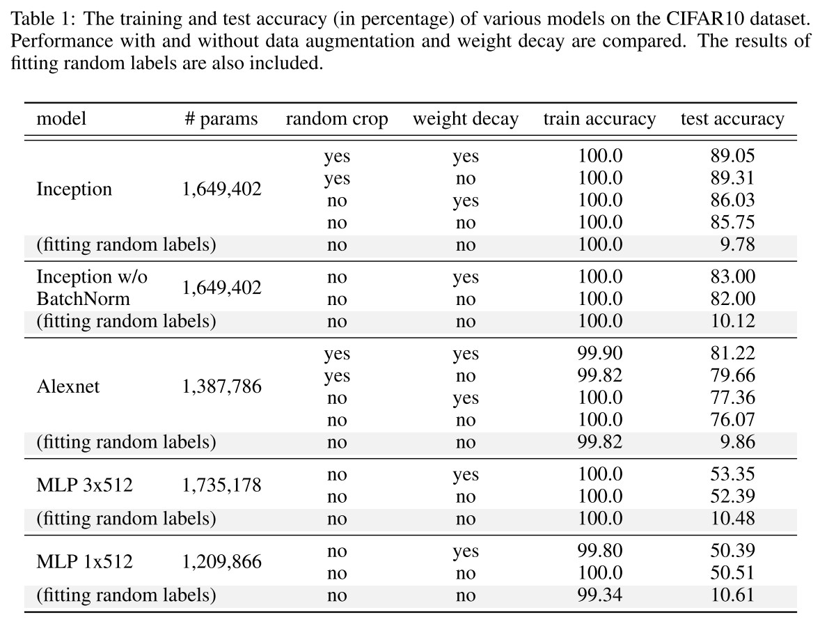
As shown in Table 1, both regularization techniques help to improve the generalization performance, but even with all of the regularizers turned off, all of the models still generalize very well.

With regularization, these models can still well fit in the random labels.

In summary, our observations on both explicit and implicit regularizers are consistently suggesting that regularizers, when properly tuned, could help to improve the generalization performance.

However, it is unlikely that the regularizers are the fundamental reason for generalization, as the networks continue to perform well after all the regularizers removed.

Finite-sample expressivity

Previous efforts on characterizing the expressivity of neural networks are almost all at the "population level", i.e. showing what functions of the entire domain can and cannot be represented by certain classes of neural networks with the same number of parameters.

With the same number of parameters, what kind of functions can be represented by certain model is the main focus on previous research over expressivity.

They argue that what is more relevant in practice is the expressive power of neural networks on a finite sample of size $n$.

Specifically, as soon as the number of parameters $p$ of a networks is greater than $n$, even simple two-layer neural networks can represent any function of the input sample.

A neural network $C$ can represent any function of a sample of size $n$ in $d$ dimensions is defined as

Theorem 1. There exists a two-layer neural network with ReLU activations and $2n+d$ weights that can represent any function on a sample of size $n$ in $d$ dimensions.

The expressivity of neural network is very powerful.

Inspirations

This paper shows an interesting discovery that a convolutional neural network can fit in random labeled data. Thus the Rademacher complexity can not explain the difference of the generalization error between different models.

Shortcut Learning in Deep Neural Networks - 2020 Perspective Article

Code: https://github.com/rgeirhos/shortcut-perspective

Robert Geirhos, Jörn-Henrik Jacobsen, Claudio Michaelis, Richard Zemel, Wieland Brendel, Matthias Bethge, Felix A. Wichmann. Shortcut Learning in Deep Neural Networks. arXiv preprint 2020. arXiv:2004.07780

See Shortcut Learning.

Frequency perspective

A Fourier Perspective on Model Robustness - NIPS 2019

Code: https://github.com/google-research/google-research/tree/master/frequency_analysis

Dong Yin, Raphael Gontijo Lopes, Jonathon Shlens, Ekin D. Cubuk, Justin Gilmer. A Fourier Perspective on Model Robustness in Computer Vision. NIPS 2019. arXiv:1906.08988

See Interprertation for Robustness and Adversarial Example.

High-frequency Component Helps Explain the Generalization of Convolutional Neural Networks - CVPR 2020

Code: https://github.com/HaohanWang/HFC

Haohan Wang, Xindi Wu, Pengcheng Yin, Eric P. Xing. High-frequency Component Helps Explain the Generalization of Convolutional Neural Networks. CVPR 2020. arXiv:1905.13545

We first notice CNN’s ability in capturing the high-frequency components of images.

Obviously not first....

They investigate the relationship between the spectrum of image data and the generalization behavior of convolutional neural networks (CNN).

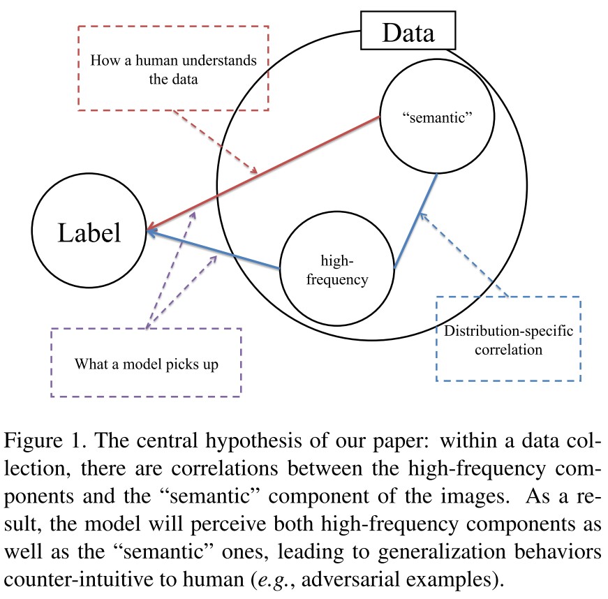
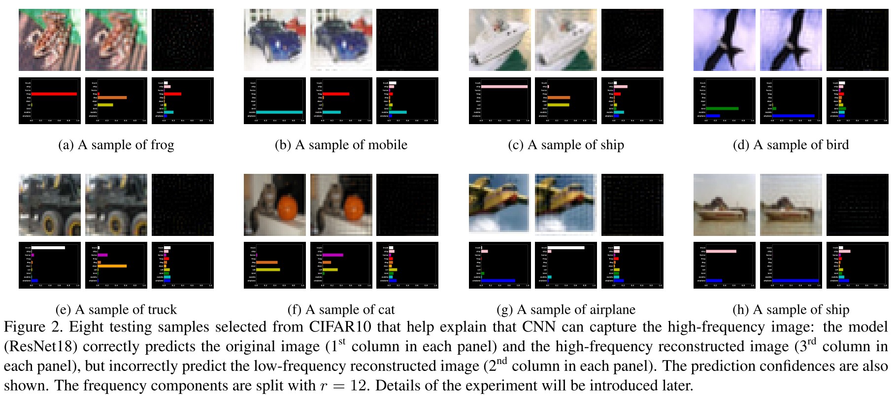
We suggest that the unintuitive generalization behaviors of CNN as a direct outcome of the perceptional disparity between human and models (as argued by Figure 1): CNN can view the data at a much higher granularity than the human can.

CNN can exploit the high-frequency image components that are not perceivable to human.

As shown in Figure 2, for these examples, the prediction outcomes are almost entirely determined by the high-frequency components of the image, which are barely perceivable to human.

Notations

They use the following notations:

• $\left<x,y\right>$, a data sample
• $f(\cdot;\theta)$, a convolutional neural network parameterized by $\theta$
• $f(\cdot;\mathcal{H})$, the human classifier (i.e. how human classifies the data)
• $l(\cdot,\cdot)$, a generic loss function (e.g. cross-entropy loss)
• $\alpha(\cdot,\cdot)$, a function evaluating prediction accuracy (1 for correctly classified sample and 0 otherwise)
• $d(\cdot,\cdot)$, a function evaluating the distance between two vectors
• $\mathcal{F}(\cdot)$, $\mathcal{F}^{-1}(\cdot)$, the Fourier transform and its inverse
• $z=\mathcal{F}(x)$, the frequency component of a sample

In this paper, we simply discard the imaginary part of the results of $\mathcal{F}^{-1}(\cdot)$ to make sure the resulting image can be fed into CNN as usual.

CNN exploit high-frequency components

They first decompose the raw data into low-frequency and high-frequency components, denoted as LFC and HFC respectively:

acquired by a radius filter $t(\cdot;r)$, i.e.

If x has more than one channel, then the procedure operates on every channel of pixels independently.

This is a trivial filter.

They assume (denoted as A1) that only $x_l$ is perceivable to human while $x_l$ and $x_h$ are both perceivable to CNN, i.e. for human:

and for CNN:

CNN may learn to exploit $x_h$ to minimize the loss. As a result, CNN’s generalization behavior appears unintuitive to a human.

For example, the adversarial examples [54, 21] can be generated by perturbing $x_h$; the capacity of CNN in reducing training error to zero over label shuffled data [65] can be seen as a result of exploiting $x_h$ and overfitting sample-specific idiosyncrasy.

Trade-off between robustness and accuracy

The accuracy of $\theta$ is

and the adversarial robustness of $\theta$ under adversarial attack bounded by $\epsilon$ is

They assume (denoted as A2) that for model $\theta$, there exists a sample $\left<x,y\right>$ such that

This assumption can be empirically verified by Figure 2.

Based on the above two assumptions, A1 and A2, they have the following corollary:

Corollary 1. With assumptions A1 and A2, there exists a sample $\left<x,y\right>$ that the model $\theta$ cannot predict both accurately and robustly under any distance metric $d(\cdot,\cdot)$ and bound $\epsilon$ as long as $\epsilon\ge d(x,x_l)$.

The proof is a direct outcome of the previous discussion and thus omitted.

If $\epsilon\ge d(x,x_l)$, it means that the adversary can craft an adversarial example using the low-frequency component, which is not correctly predicted by the model.

Rethinking Data before Rethinking Generalization

Our first aim is to offer some intuitive explanations to the empirical results observed in [65]: neural networks can easily fit label-shuffled data.

They hypothesis that Despite the same outcome as a minimization of the training loss, the model considers different level of features in the two situations:

• In the original label case, the model will first pick up LFC, then gradually pick up the HFC to achieve higher training accuracy.
• In the shuffled label case, as the association between LFC and the label is erased due to shuffling, the model has to memorize the images when the LFC and HFC are treated equally.

Experiments

We use ResNet-18 [22] for CIFAR10 dataset [33] as the base experiment.

We train two models, with the natural label setup and the shuffled label setup, denote as M_natural and M_shuffle, respectively.

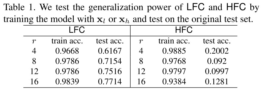
To test which part of the information the model picks up, for any $x$ in the training set, we generate the low-frequency counterparts $x_l$ with $r$ set to 4, 8, 12, 16 respectively.

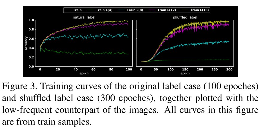
As shown in Figure 3, M_natural prefers to pick up the LFC, i.e. the very low-frequency component (filtered with a radius of 4) reaches more than 40% even at the beginning, while M_shuffle has no clear preference between LFC and HFC.

They conjecture that since the data sets are organized and annotated by human, the LFC-label association is more “generalizable” than the one of HFC: picking up LFC-label association will lead to the steepest descent of the loss surface, especially at the early stage of the training.

They also test the performance of using LFC or HFC independently for training, as shown in Table 1, LFC is much more “generalizable” than HFC.

They propose to explain the training process as picking up LFC first and than probing for HFC for better accuracy, compared with the information bottlenet theory that the model memorizes the data first and than forget the unimportant details. I think these two explanations seem intuitively contradictory.

A remaining question

The coincidental alignment between networks’ preference in LFC and human perceptual preference might be a simple result of the “survival bias” of the many technologies invented one of the other along the process of climbing the ladder of the state-of-the-art.

However, an interesting question will be how well these ladder climbing techniques align with the human visual preference.

Questioning the metric.

Training heuristics

We test multiple heuristics by inspecting the prediction accuracy over LFC and HFC with multiple choices of $r$ along the training process and plot the training curves.

They evaluate the model's performance on LFC and HFC under various batch size, and following tricks (heuristics):

• Dropout: A heuristic that drops weights randomly during training.
• Mix-up: A heuristic that linearly integrate samples and their labels during training.
• BatchNorm: A method that perform the normalization for each training mini-batch to accelerate Deep Network training process.
• Adversarial Training: A method that augments the data through adversarial examples generated by a threat model during training.

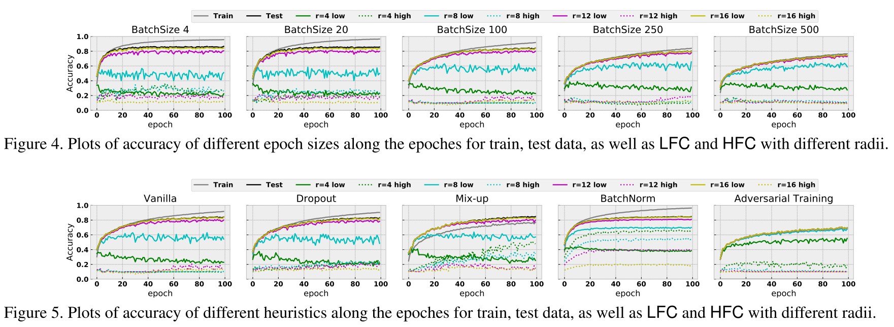
As shown in Figure 4, smaller batch size appears to excel in improving training and testing accuracy, while bigger batch size seems to stand out in closing the generalization gap.

The train and test accuracy is higher with smaller batch size, but their difference is also larger with smaller batch size.

Intuitively, with bigger epoch size, the features that can lead to steepest descent of the loss surface are more likely to be the “generalizable” patterns of the data, which are LFC.

With larger batch size, the model is more invariant to HFC.

As shown in Figure 5:

• Dropout roughly behaves similarly to the vanilla set-up in our experiments.

• Mix-up delivers a similar prediction accuracy, however, it catches much more HFC.

• Adversarial training mostly behaves as expected: it reports a lower prediction accuracy, which is likely due to the trade-off between robustness and accuracy.

  It seems that adversarial training biases the model towards low-frequency components and results a smaller generalization gap.

  However, adversarial training seems to be sensitive to the HFC when $r=4$, which is ignored even by the vanilla set-up.

• The performance of BatchNorm is notable: compared to the vanilla set-up, BatchNorm picks more information in both LFC and HFC.

They test different model architectures, including LeNet, AlexNet, VGG and ResNet, discover that the ResNet resulrs better vanilla test accuracy, smaller generalization gap and a weaker tendency in capturing HFC.

They test different optimizers, including SGD, ADAM, AdaGrad, AdaDelta and RMSprop, and notice that SGD seems to be the only one suffering from the tendency towards significantly capturing HFC.

A hypothesis on Batch Normalization

We hypothesized that one of BatchNorm’s advantage is, through normalization, to align the distributional disparities of different predictive signals.

They hypothesize that BatchNorm align the magnitudes of different predictive signals, e.g. HFC is generally smaller than LFC and BatchNorm can help.

To verify this hypothesis, we compare the performance of models trained with vs. without BatchNorm over LFC data and plot the results in Figure 6.

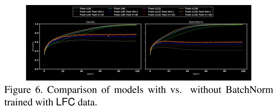
As shown in Figure 6, when the model is trained with only LFC, BatchNorm does not always help improve the predictive performance, either tested by original data or by corresponding LFC data.

Smooth kernels and robustness

Robust model tends to have smoother kernels.

This has been observed before.

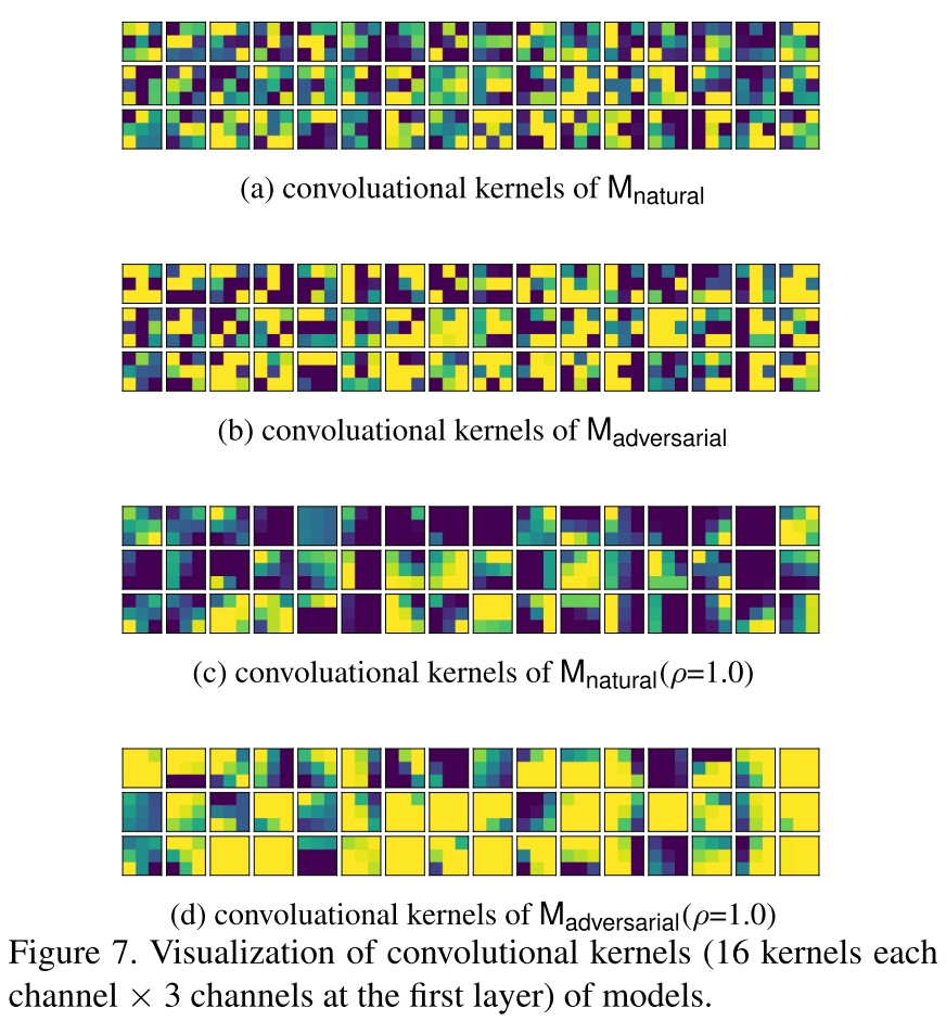
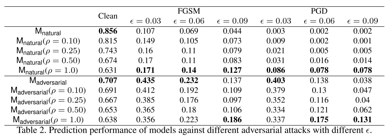
They propose a simple kernel smoothing method, i.e.

where $\mathcal{N}(i,j)$ is the set of the spatial neighbors of $(i,j)$ and $\rho$ is a hyperparameter, and find that it can increase robustness as shown in Table 2.

The improvement is actually marginal, same as the results I obtained myself.

Beyond image classification

They also test on the RetinaNet with ResNet50+FPN on MS COCO dataset.

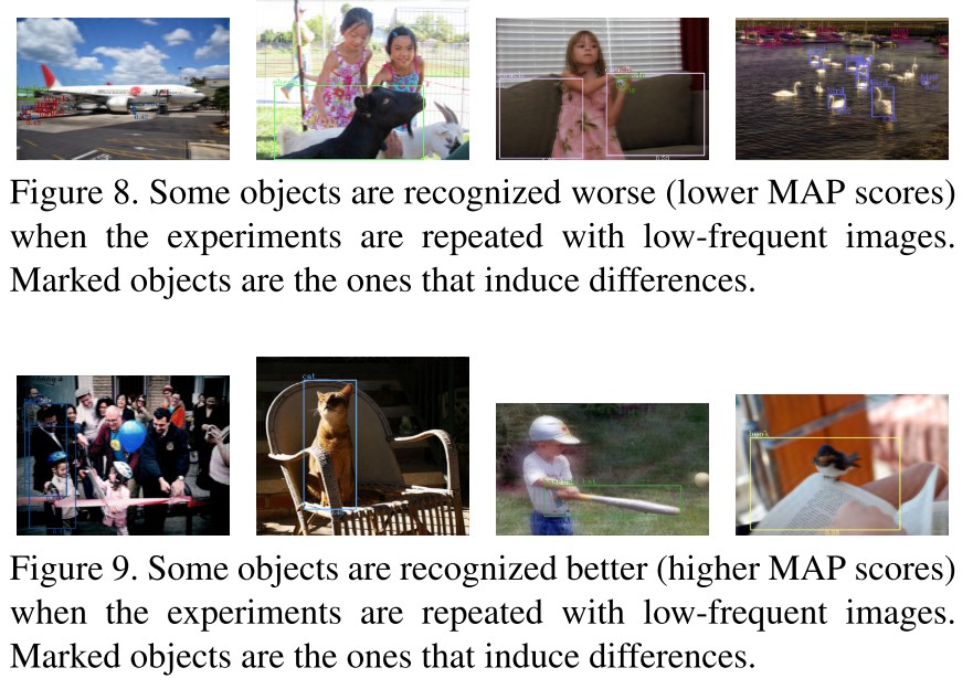
They find that the performance drops on some $x_l$, and explain that $x_l$ may not have rich enough information when HFC are dropped as shown in Figure 8.

Also, the MAP increases on some $x_l$ as shown in Figure 9.

There seems no apparent reasons why these objects are recognized better in low-frequent images, when inspected by human.

Are HFC just noises?

They decompose the images using SVD and reconstruct them respectively using dominant singular and trailing singulars, and

With this set-up, we find much fewer images supporting the story in Figure 2.

Our observations suggest the signal CNN exploit is more than just random “noises”.

Future

They give some suggestions on the future research in computer vision:

• A single numeric on the leaderboard, while can significantly boost the research towards a direction, does not reliably reflect the alignment between models and human, while such an alignment is arguably paramount.

  Dismiss the SOTA trending....

• We hope our work will set forth towards a new testing scenario where the performance of low-frequent counterparts needs to be reported together with the performance of the original images.

  Test whether the model is biased to HFC.....

• Explicit inductive bias considering how a human views the data (e.g., [58, 57]) may play a significant role in the future. In particular, neuroscience literature have shown that human tend to rely on low-frequent signals in recognizing objects [4, 5], which may inspire development of future methods.

  Look for more human-like metric...

Inspirations

This paper is quite informative, although most of the phenomena they listed are not novel before this paper. A comprehensive analysis over these phenomena is still a remarkable contribution that they made in this paper.

They explain the training process of a deep learning model as picking up low-frequency components first and then probing high-frequency components for higher accuracy, leading the major disparity between human perception and model.

They also show that many heuristic tricks (e.g. mix-up, batchnorm) exploit the high-frequency components for a better accuracy, which is misaligned with human perception. A smaller batch size also encourages relatively more focus on high-frequency component compared with a larger one. Adversarial training encourages the model to focus more on low-frequency components.

The adversarial vulnerability may root from the model's dependence on high-frequency components and they also show that if the low-frequency component of some example is a natural adversarial example under the given threat model, the model cannot acquire both accuracy and robustness on this example under the same threat model.

I think the following are possible followups:

• For a certain dataset, is it possible to acquire remarkable robustness using LFC?

• Can we give a principle on how low the low-frequency component should be to maintain the information?

  How to decompose an example's robust and non-robust feature? Are they LFC and HFC respectively?

• The explanation of the training process is different from that of the information bottleneck theory, can we reconcile them? (although the information bottleneck theory is disputable by itself)

• Why ResNet has a weaker tendency on capturing HFC?

• Why some LFC of some objects can increase the MAP?

Tricks

When Does Label Smoothing Help? - NIPS 2019

Rafael Müller, Simon Kornblith, Geoffrey Hinton. When Does Label Smoothing Help? NIPS 2019. arXiv:1906.02629

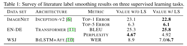
The generalization and learning speed of a multi-class neural network can often be significantly improved by using soft targets that are a weighted average of the hard targets and the uniform distribution over labels.

Szegedy et al. [6] introduced label smoothing, which improves accuracy by computing cross entropy not with the “hard" targets from the dataset, but with a weighted mixture of these targets with the uniform distribution.

Here we show empirically that in addition to improving generalization, label smoothing improves model calibration which can significantly improve beam-search.

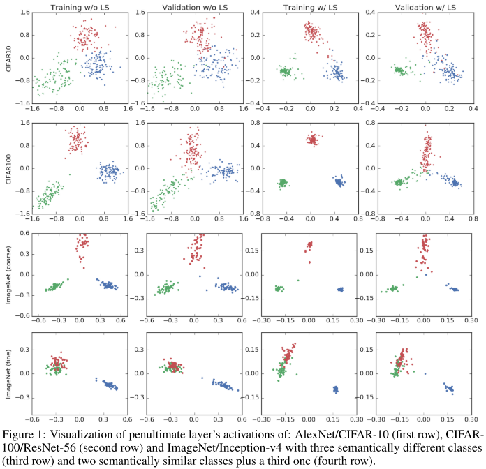
We show that label smoothing encourages the representations of training examples from the same class to group in tight clusters.

Label smoothing

The prediction of a neural network written as a function of the activations in the penultimate (倒数第二) layer is

in which:

• $p_k$, the predicted likelihood that the input is classified as the $k$-th class by the model
• $w_k$, the weights and biases of the last layer
• $x$, the vector containing the activations of the penultimate layer of a neural network concatenated with "1" to account for the bias

For a network trained on "hard" labels, the objective is the expected value of the cross-entropy between the true targets $y_k$ and the network's outputs $p_k$, i.e.

For a network trained with a label smoothing of parameter $\alpha$, the objective is instead the cross-entropy between the modified targets $y_k^{LS}=y_k(1-\alpha)+\alpha/K$ and the networks' outputs $p_k$.

The label is not either 1 or 0, it's softened among all targets.

Penultimate layer representations

The logit of the $k$-th class, i.e. $x^\top w_k$ can be thought of as a measure of the squared Euclidean distance between the activations of the penultimate layer $x$ and a template $w_k$, since

where $x^\top x$ is factored out when calculating the softmax outputs, and $w_k^\top w_k$ is usually constant across classes, hence each class has a template $w_k$.

A new perspective on the inference of neural networks, it now becomes a combination of template match, shift and non-linear transformations.

Therefore, label smoothing encourages the activations of the penultimate layer to be close to the template of the correct class and equally distant to the templates of the incorrect classes.

For a hard label, incorrect classes is labeled as zero, which leaves the distance of the representation to the templates of incorrect classes unconstrained.

They propose a new scheme to observe this property of label smoothing:

1. Pick three classes
2. Find an orthonormal basis of the plane crossing the templates of these three classes
3. Project the penultimate layer activation of examples from these three classes onto this plane

Three templates form a plane with two ratios along each basis, with which one can project the representation onto a reasonable 2-D subspace.

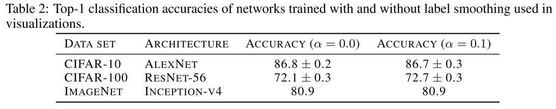
As shown in Figure 1, they validate this hypothesis on ImageNet, CIFAR-100 and CIFAR-10, the last two columns are trained with a label smoothing factor of 0.1.

Therefore, when looking at the projections, the clusters organize in regular triangles when training with label smoothing, whereas the regular triangle structure is less discernible in the case of training with hard-targets (no label smoothing).

Finally, we test our visualization scheme in an Inception-v4/ImageNet experiment and observe the effect of label smoothing for semantically similar classes.

We also observe that when training without label smoothing there is continuous degree of change between the "tench" cluster and the "poodles" cluster. We can potentially measure "how much a poodle is a particular tench". However, when training with label smoothing this information is virtually erased.

The indicates that label should be weighted according to the semantical similarity among classes.

Implicit model calibration

But does it improve the calibration of the model by making the confidence of its predictions more accurately represent their accuracy?

Here, we show that label smoothing also reduces ECE (Expected Calibration Error) and can be used to calibrate a network without the need for temperature scaling.

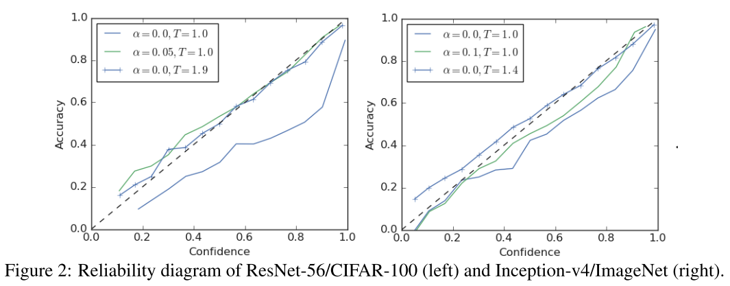
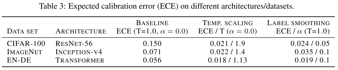
As shwon in Figure 2, a vanilla model is over confident as the solid blue line implies, with proper calibration using a temperature of 1.9, or using a label smoothing with a factor of 0.05, the model is both calibrated.

This is also revealed in the visualization in Figure 1, besides a more tight cluster in the training set, in the validation set it spreads towards the center representing the full range of confidences for each prediction.

They also show similar conclusions on NLP tasks.

It's omitted here.

Knowledge distillation

We show that, even when label smoothing improves the accuracy of the teacher network, teachers trained with label smoothing produce inferior student networks compared to teachers trained with hard targets.

In knowledge distillation, the cross-entropy term $H(\bold{y},\bold{p})$ is replaced by the weighted sum written as

in which, $p^t_k(T)$ and $p_k(T)$ are the outputs of teacher and student after temperature scaling with $T$ and $\beta$ controls the balance between two tasks:

• fitting the hard-targets
• approximating the softened teacher

If $\beta=1$, then the knowledge distillation becomes training the student model with smooth label weighted by the experience of the teacher model.

They consider four results:

1. the teacher’s accuracy as a function of the label smoothing factor
2. the student’s baseline accuracy as a function of the label smoothing factor without distillation
3. the student’s accuracy after distillation with temperature scaling to control the smoothness of the teacher’s provided targets (teacher trained with hard targets)
4. the student’s accuracy after distillation with fixed temperature (T = 1.0 and teacher trained with label smoothing to control the smoothness of the teacher’s provided targets)

They define an equivalent label smoothing factor $\gamma$.

• for scenarios 1 and 2, $\gamma=\alpha$.
• for scenarios 3 and 4, $\gamma=\Bbb{E}[\sum_{k=1}^K(1-y_k)p_k^t(T)K/(K-1)]$, i.e. the confidence of the teacher allocated to incorrect examples over the training set.

They consider only the case where $\beta=1$.

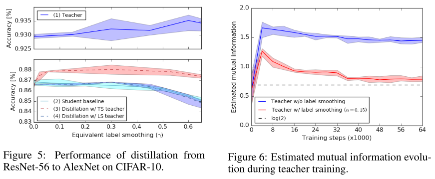
As shown in Figure 5,

For this particular setup, increasing α improves the teacher’s accuracy up to values of α = 0.6, while label smoothing slightly degrades the baseline performance of the student networks.

The figure shows that using these better performing teachers is no better, and sometimes worse, than training the student directly with label smoothing, as the relative information between logits is "erased" when the teacher is trained with label smoothing.

Therefore, a teacher with better accuracy is not necessarily the one that distills better.

A good teacher should tolerate with its own error somehow?

Fig. 6 shows the estimated mutual information between a subset (N = 600 from two classes) of the training examples and the difference of the logits corresponding to these two classes.

The mutual information is calculated between the input and the logits. The original form of mutual information between two distributions is

and they approximate it with

in which:

• $X$ is a discrete variable representing the index of the training example
• $Y$ is continuous representing the difference between two logits, which they estimate as a Gaussian
• $z_x$ is the flattened input image indexed by $x$
• $d(\cdot)$ is a random data augmentation function (e.g. random shift)
• $f(\cdot)$ is a trained neural network with an image as an input and the difference between two logits as output
• $\mu_x=\sum_{l=1}^L f(d(z_x))/L$, $L$ is the number of Monte Carlo samples used to calculate the mean
• $\sigma^2=\sum_{x=1}^N (f(d(z_x))-\mu_x)^2/N$, $N$ is the number of training examples used fro mutual information estimation

As the representations collapse to small clusters of points, much of the information that could have helped distinguish examples is lost.

In this case, all the information of the input is discarded except a single bit representing which class the example belongs to, resulting in no extra information in the teacher’s logits compared to the information in the labels.

It seems that teachers trained with label smoothing results to provide information no more than that provided by the original labels. So, in this case, the students may as well learn from the labels directly?

Inspirations

They offer a nice visualization explaining the effect of label smoothing, well it can be either viewed as a confidence penalty, or a prior teacher. It appears that with label smoothing, the representations learned tend to be more clustered and more equally distributed, while the information coded in representation of different examples varies less (since it's more tightly centered).

I think a proper reweight of label smoothing will be more adequate, but, since the teacher can offer a learned distribution of labels, it seems that it's quite redundent. The problem of a hard label stems from the characteristic that zero surves as a zero element in multiplication, making the representation learned only focuses on the cluster itself, without constraining its distance to other clusters.