Interpretation for Robustness and Adversarial Example

By LI Haoyang 2020.11.2

Content

Empirical work

A Fourier Perspective on Model Robustness - NIPS 2019

Code: https://github.com/google-research/google-research/tree/master/frequency_analysis

Dong Yin, Raphael Gontijo Lopes, Jonathon Shlens, Ekin D. Cubuk, Justin Gilmer. A Fourier Perspective on Model Robustness in Computer Vision. NIPS 2019. arXiv:1906.08988

We find that both methods improve robustness to corruptions that are concentrated in the high frequency domain while reducing robustness to corruptions that are concentrated in the low frequency domain.

They aim to probe the following question

What is different about the corruptions for which augmentation strategies improve performance vs. those which performance is degraded?

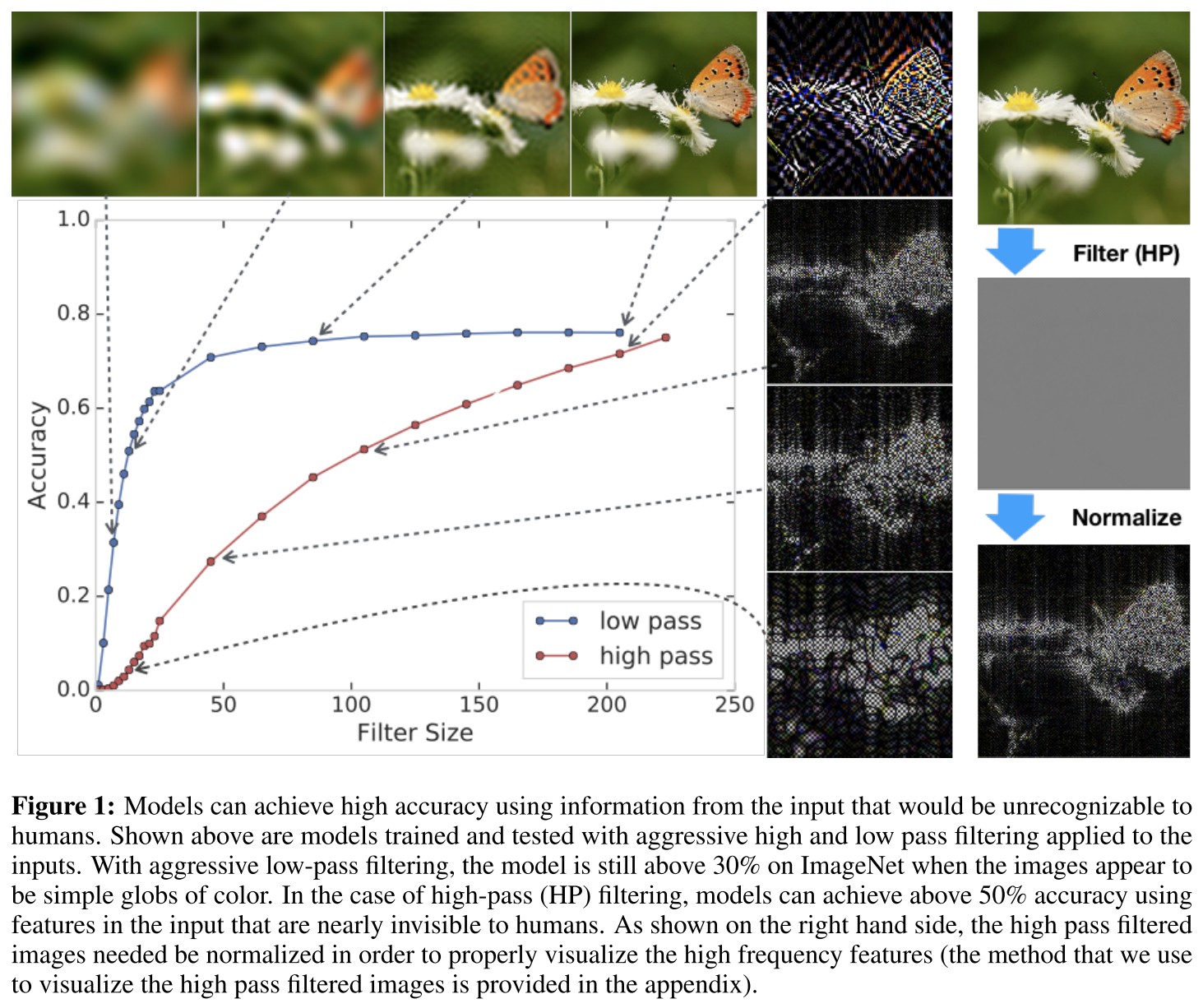
Accuracy of model under filters

For our experiments on CIFAR-10, we use the Wide ResNet-28-10 architecture [27], and for our experiment on ImageNet, we use the ResNet-50 architecture [16].

All experiments use flip and crop during training.

The model can still achieve a relatively high accuracy when the input image is aggressively filtered.

Effect of data augmentation to models in a Fourier perspective

Ford et al. [10] investigated the robustness of three models on CIFAR-10-C: a naturally trained model, a model trained by Gaussian data augmentation, and an adversarially trained model. It was observed that Gaussian data augmentation and adversarial training improve robustness to all noise and many of the blurring corruptions, while degrading robustness to fog and contrast.

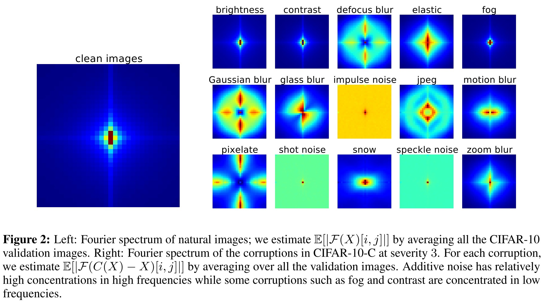
As shown in Figure 2, the right are the spectrum of different noises, it's obvious that the corruption by fog and contrast highly corrupts the low frequency components in the image. This suggests that the Gaussian data augmentation and avdersarial training encourages the model to focus more on low frequency information.

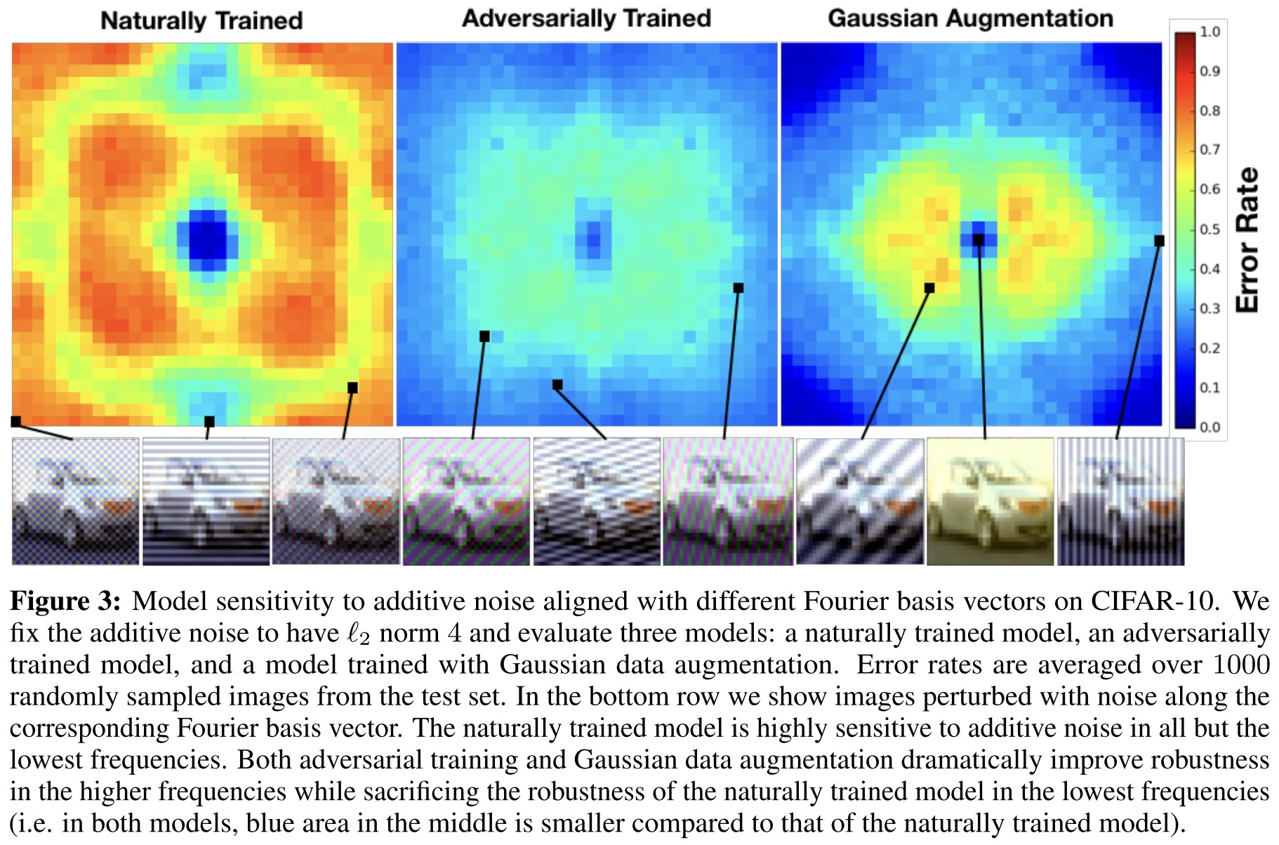
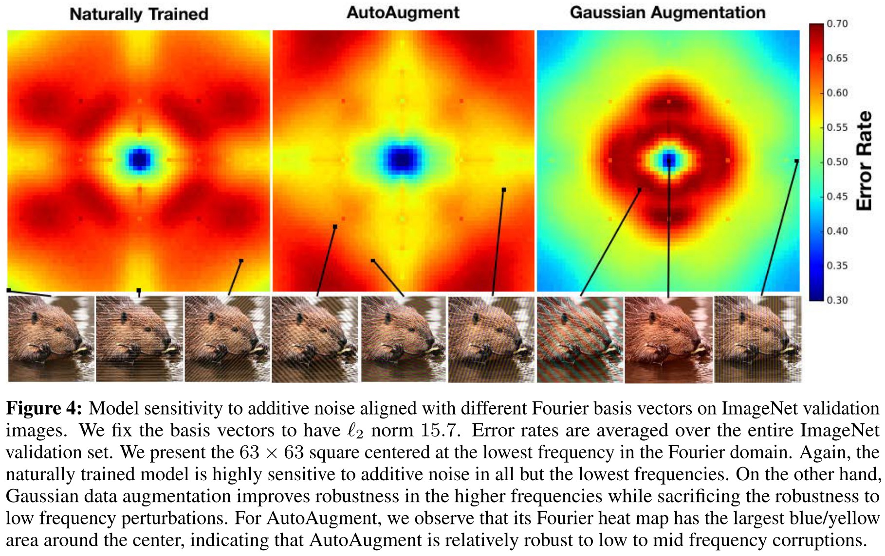
The naturally trained model is highly sensitive to additive perturbations in all but the lowest frequencies, while Gaussian data augmentation and adversarial training both dramatically improve robustness in the higher frequencies.

A weird result is that augmenting the model with fog noise does not improve its performance on fog corrupted data.

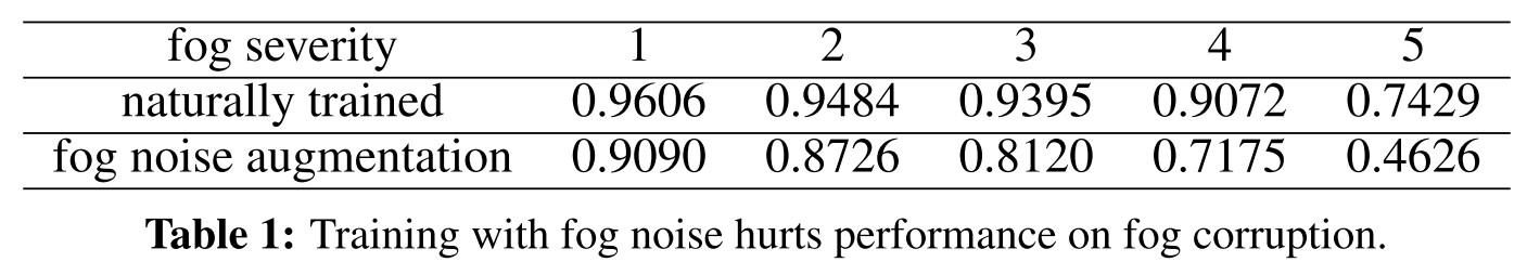
It's not aligned with intuition.

Adversarial examples are not strictly a high frequency phenomenon

A common hypothesis is that adversarial perturbations lie primarily in the high frequency domain. In fact, several (unsuccessful) defenses have been proposed motivated specifically by this hypothesis. Under the assumption that compression removes high frequency information, JPEG compression has been proposed several times [21, 2, 7] as a method for improving robustness to small perturbations.

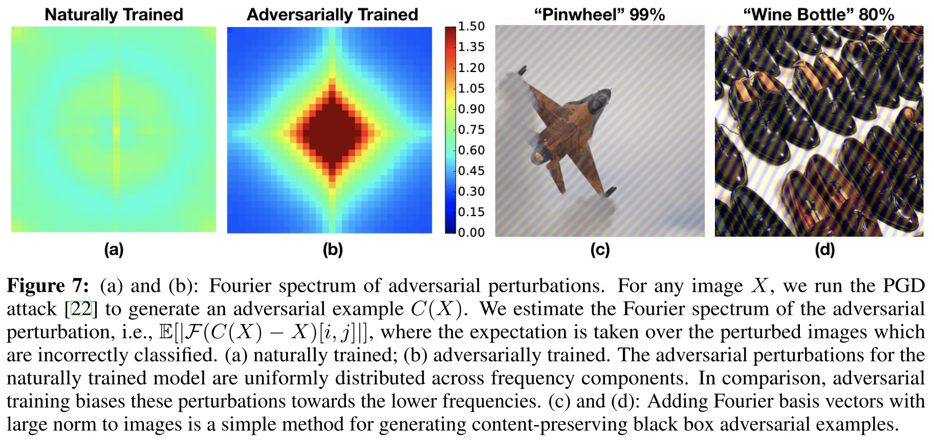
They observe that adversarial perturbations generated for naturally trained model show higher concentrations on higher frequency domain, while those for adversarially trained model resemble that of a natural image.

The fact that adversarial training biases these perturbations towards the lower frequencies suggests an intriguing connection between adversarial training and the DeepViz [23] method for feature visualization.

Perhaps the reason adversarially trained models have semantically meaningful gradients [25] is because gradients are biased towards low frequencies in a similar manner as utilized in DeepViz.

We observe that adding certain Fourier basis vectors with large norm (24 for ImageNet) degrades test accuracy to less than 10% while preserving the semantics of the image.

Inspirations

This paper shows that adversarially trained models focus more on low frequency information as well as Gaussian augmented trained models, and it's possible to perturb in frequency domain with mild noise to craft an adversarial example, which is a potential way for single-query black-box adversarial attack.

Following this direction, the Jacobian regularized network is an expected work.

Interpreting Adversarially Trained Convolutional Neural Networks - ICML 2019

Code: https://github.com/PKUAI26/ATCNN

Tianyuan Zhang, Zhanxing Zhu. Interpreting Adversarially Trained Convolutional Neural Networks. ICML 2019. arXiv:1905.09797

Surprisingly, we find that adversarial training alleviates the texture bias of standard CNNs when trained on object recognition tasks, and helps CNNs learn a more shape-biased representation.

Our findings shed some light on why AT-CNNs are more robust than those normally trained ones and contribute to a better understanding of adversarial training over CNNs from an interpretation perspective.

They attempt to find the differences that the "robustness" brings to the network, and discover that the "robust" model relies more on shapes rather than textures and results a more interpretable prediction.

Salience map

The visualized salience map $E\in\R^d$ aims to show the sensitivity of the output to each pixel of an input image.

Salience methods can mainly be divided into:

• Perturbation-based methods
• Gradient-based methods

The recent sanity check filters out only variants of Grad and GradCAM.

A trained network $f:\R^d\to\R^K$ maps an input image $x\in\R^d$ of $d$ dimensions to $K$ classes.

Let $S_c$ denotes the class activation function for each class $c$, the Grad explanation is the gradient of class activation with respect to the input image $x$, i.e.

SmoothGrad is proposed to alleviate noises in gradient explanation by averaging over the gradient of noisy copies of an input, i.e.

They choose $S_c(x)=\text{log}p_c(x)$, i.e. the log of the probability of class $c$ assigned by a classifier to input $x$.

It's no different from the generating of adversarial examples very much, although the latter acquires the perturbed example rather than the perturbation itself.

Distortions

They decide to check the degradation of AT-CNN and CNN under severe distortion of different features.

The distortions used consist of the following

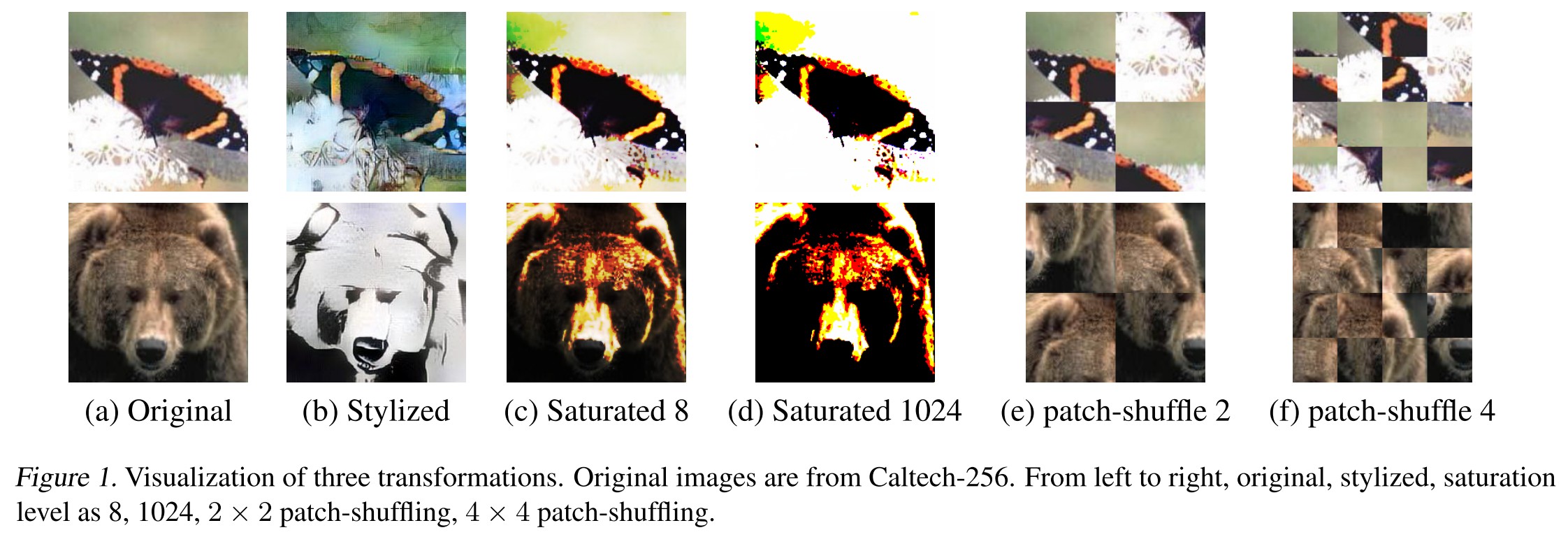
• Stylizing

  We utilize style transfer to destroy most of the textures while preserving the global shape structures in image.

• Saturation

  For a pixel of value $v\in[0,1]$, the saturated pixel value $x^p$ with saturation level $p$ is calculated by

  $$x^{p}=\text{sign}(2v-1)|2v-1|^{\frac{2}{p}}/2+1/2$$

  Increasing saturation level can gradually destroy some texture information while preserving most parts of the contour structures.

• Patch-Shuffling

  To destroy long-range shape information, we split images into $k\times k$ small patches and randomly.

  This operation preserves most of the texture information and destroys most of the shape information.

Experiments

Baseline performance

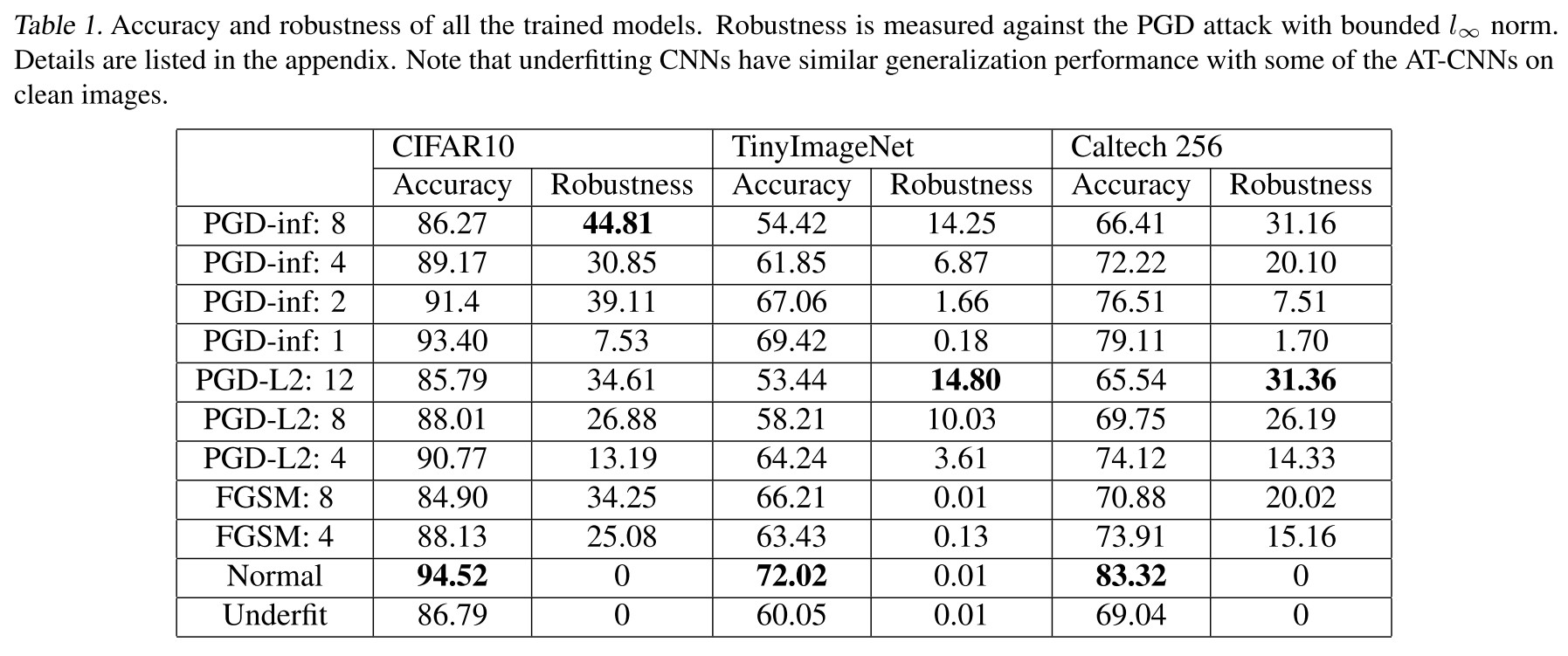
Three image datasets are considered, including Tiny ImageNet2, Caltech-256 (Griffin et al., 2007) and CIFAR-10.

When training on CIFAR-10, we use the ResNet-18 model (He et al., 2016a;b);

For both Tiny ImageNet and Caltech-256, we use ResNet-18 model as the network architecture.

Salience maps

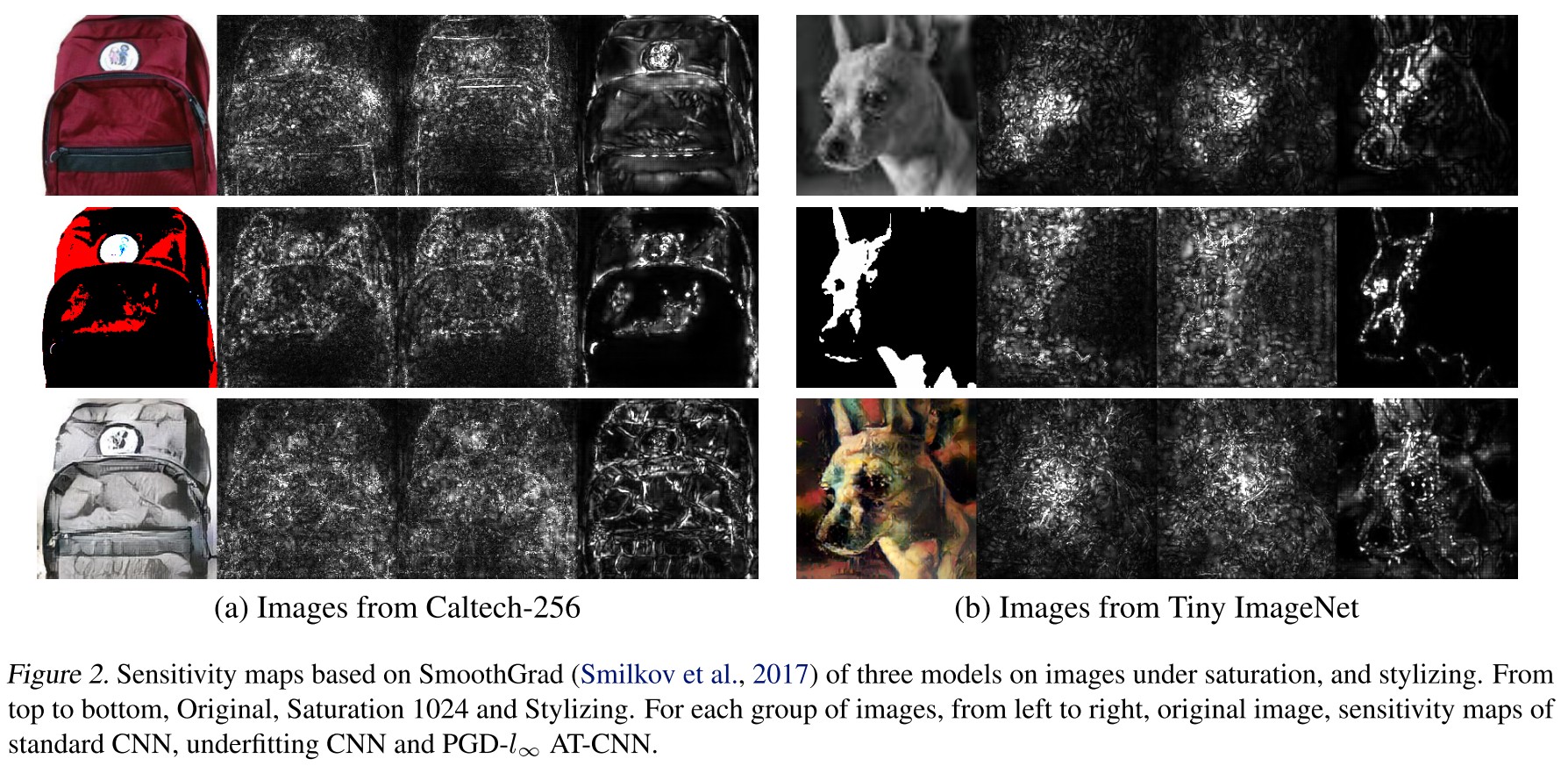
As shown in Figure 2, AT-CNN mainly focuses on the shape information of the input image.

Generalization under distortions

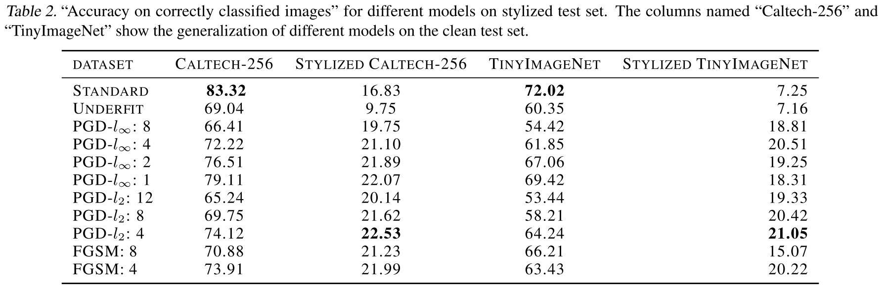
....though with a lower accuracy on original test images, AT-CNNs achieve higher accuracy on stylized ones with textures being dramatically changed.

....with the increasing level of saturation, more texture information is lost. Favorably, adversarially trained models exhibit a much less sensitivity to this texture loss, still obtaining a high classification accuracy.

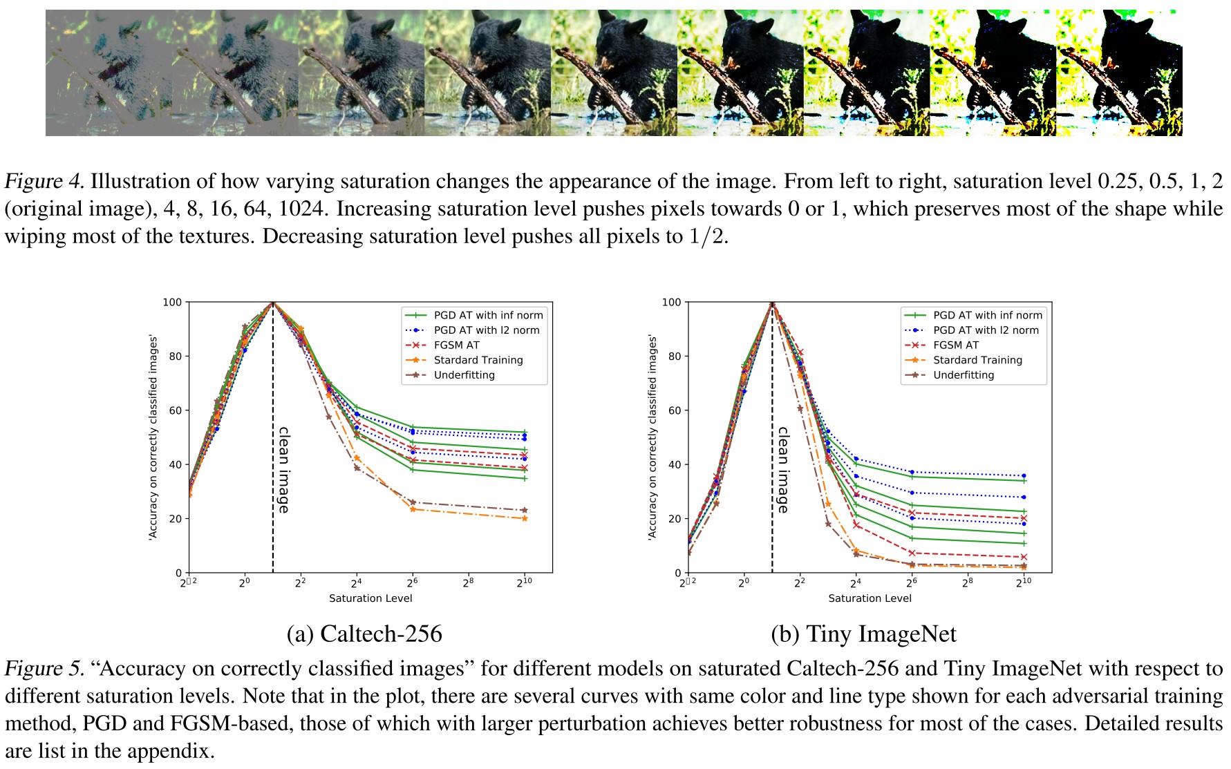
....for each adversarial training approach, either PGD or FGSM based, AT-CNNs with higher robustness towards PGD adversary are more invariant to the increasing of the saturation level and texture loss.

....indicating that ATCNNs are not robust to all kinds of image distortions. They tend to be more robust for fixed types of distortions. We leave the further investigation regarding this issue as future work.

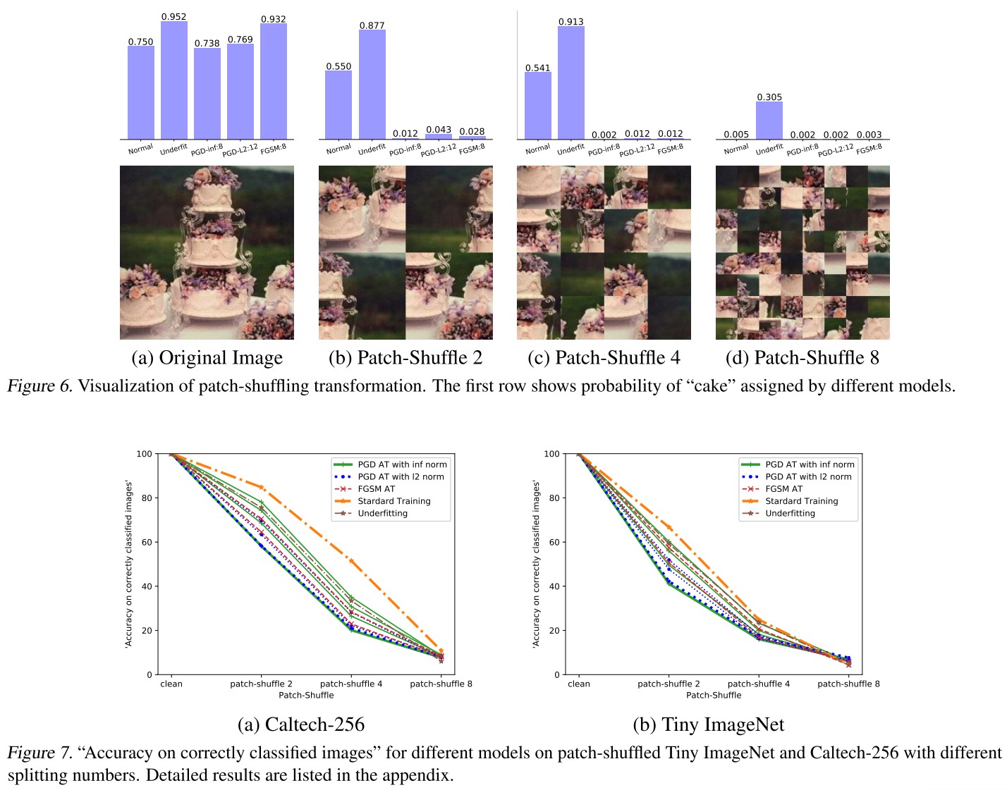
....while the normal CNNs still maintains a high confidence over the ground truth class. This reveals AT-CNNs are more baised towards shapes and edges than normally trained ones.

Discussion

This naturally raises the question: whether any other models that can capture more global features or with more texture invariance could lead to more robustness to adversarial examples, even without adversarial training?

Inspirations

This paper empirically shows that adversarially trained network focuses more on the shape information rather than texture, and points out that potentially one can enhance the robustness of model by forcing it focus more on global features. This can partially explain the performance of feature denoising.

Again, following this trajectory, JARN is an expected work.

Intriguing Properties of Adversarial Training at Scale - ICLR 2020

Paper: https://openreview.net/forum?id=HyxJhCEFDS¬eId=rJxeamAAKB

Cihang Xie, Alan Yuille. Intriguing Properties of Adversarial Training at Scale. ICLR 2020.

They discover two intriguing properties in adversarial training at scale:

• Batch Normalization may prevent networks from obtaining strong robustness in adversarial training.
• The current "deep" network are still shallow for the task of adversarial training.

The first is very natural since previous works have discovered that batch normalization will make the network tend to focus more on high frequency information, which is also proved to be less used by adversarially trained models.

The second is a little anti-intuitive since local linearity has been declared to be useful for adversarial training, and if the model should be more linear to gain robustness, and given that a deeper network is easier to overfit, i.e. produce a more non-linear boundary, it seems more rational that a more shallow network is better?

Experimental setting

Adversarial training pipeline: https://github.com/facebookresearch/ImageNet-Adversarial-Training

The basic loss function in adversarial training they used is branched from the initial proposed by Goodfellow, i.e.

In which, $J(\cdot)$ is the loss function and the training pairs $\{x^{clean},x^{adv}\}$ are composed of clean images and their corresponding adversarial examples.

The effect of clean images in adversarial training

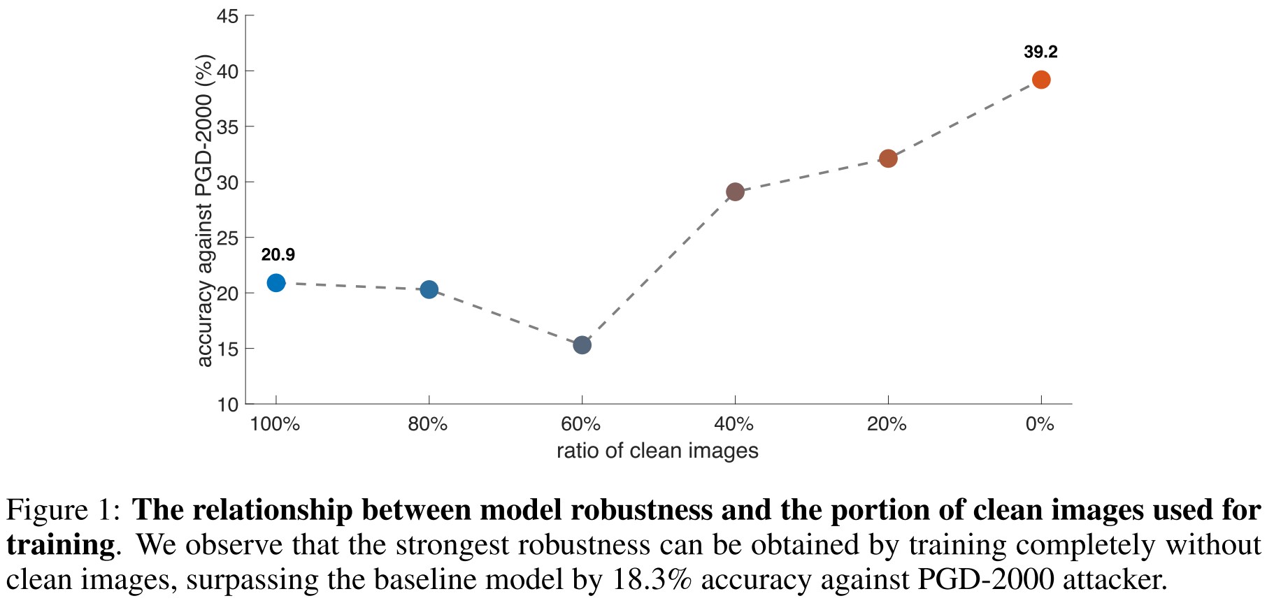
Interestingly, removing a portion of clean images from training data can significantly improve model robustness, and the strongest robustness can be obtained by completely removing clean images from the training set.

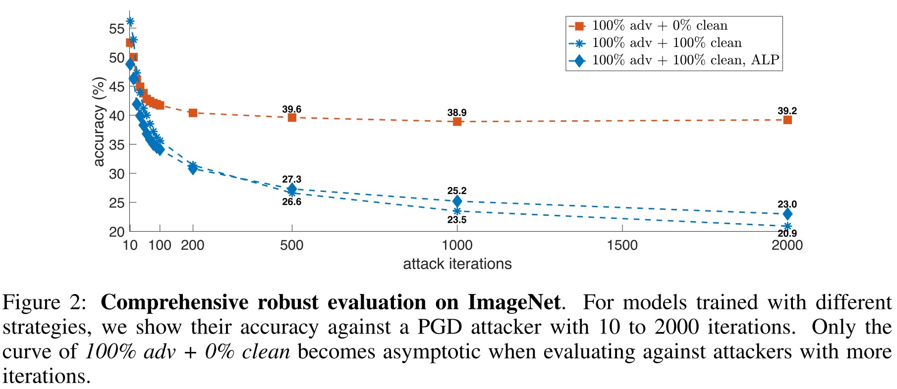
As shown in Figure 2, our re-implemented ALP obtains an accuracy of 23.0% against PGD-2000 attacker2, which outperforms the baseline model by 2.1%. Compared with the strategy of removing clean images, this improvement is much smaller.

Given the results above, we conclude that training exclusively on adversarial images is the most effective strategy for boosting model robustness.

This experiments show that training on a mixture of clean and adversarial examples obstacles the robustness performance of the resulted model.

Batch normalization in adversarial training

They hypothesis that clean images and adversarial images are drawn from different domains, i.e. sampled from different distributions. Since the parameters in Batch Normalization layers are distribution-aware (i.e. the average and deviation is sensitive to the distribution of inputs), they propose to handle clean images and adversarial examples separately in BN layers.

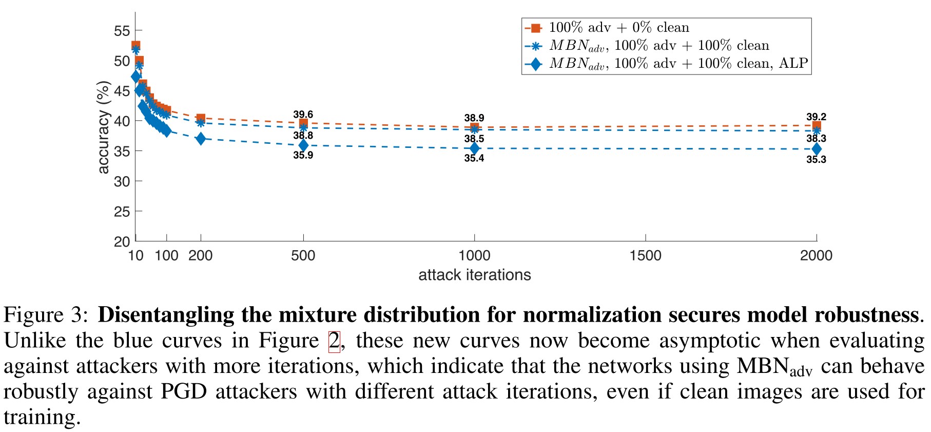
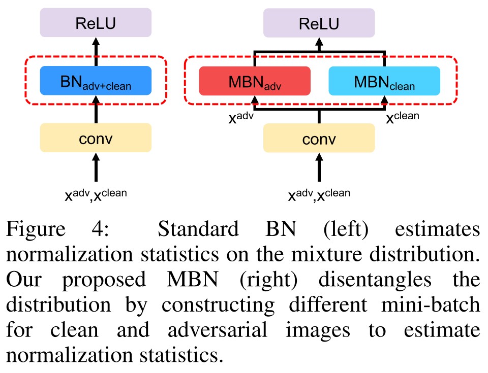
The proposed Mixture BN (MBN) appears to draw the robustness of mixed adversarially trained models to the level of that trained sole on adversarial examples, as shown in Figure 3.

In inference, they simply drop one of the MBNs.

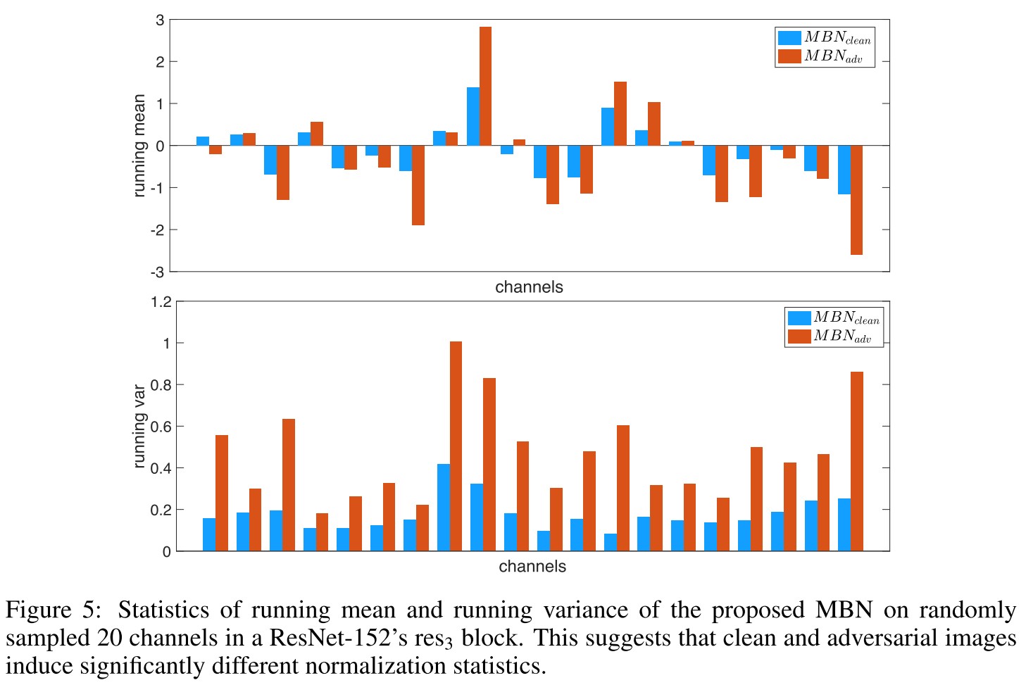
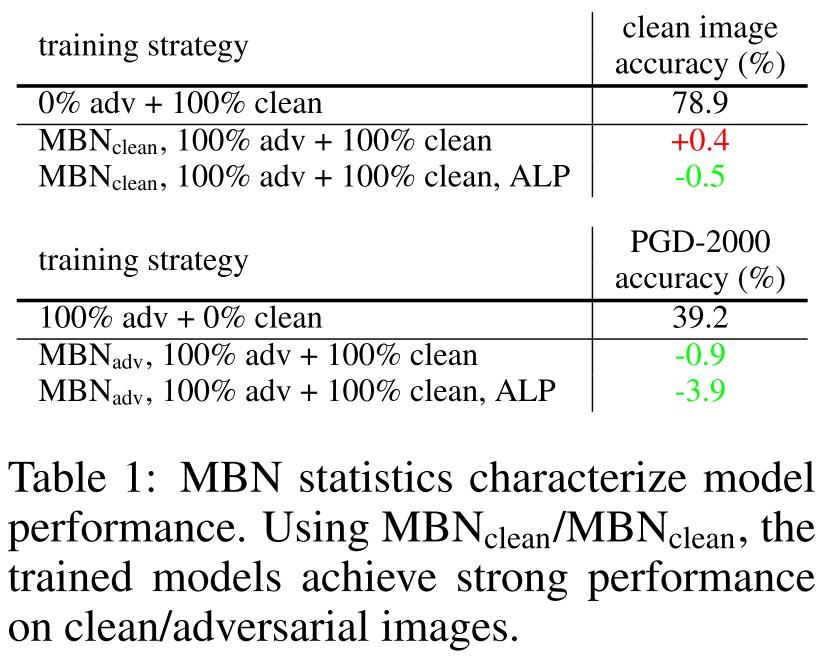
In Figure 5, they draw some characteristics of the two MBNs and verified their differences. They find that the characteristics of MBN affects the performance of the model in terms of standard accuracy or robust accuracy as shown in Table 1, and concludes

• Clean images and adversarial images come from two different domains
• Current networks fail to learn a unified representation for both domains

They also test Group Normalization, which treats each example independently, it's also effective in handling this problem.

(Kannan et al., 2018; Mosbach et al., 2018) also show that adversarial training with clean images can secure robustness on small datasets, i.e., MNIST, CIFAR-10 and Tiny ImageNet.

Intuitively, generating adversarial images on these much simpler datasets or under a smaller perturbation constraint induces a smaller gap between these two domains, and therefore making it easier for networks to learn a unified representation on clean and adversarial images.

The batch normalization behaves inconsistently in inference and training since there is no "batch" in inference.

• During training, the mean and variance are computed on each mini-batch, referred to as batch statistics.
• During testing, there is no actual normalization performed —BN uses the mean and variance pre-computed on the training set (often by running average) to normalize data, referred to as running statistics.

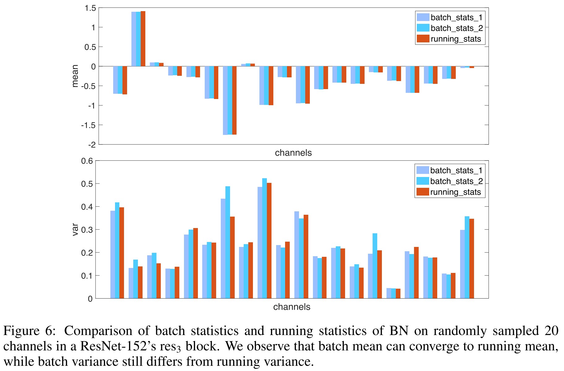
And this inconsistency is more severe in the presence of adversarial examples, as shown in Figure 6, batch mean is almost equivalent to running mean, while batch variance does not converge to running variance yet on certain channels.

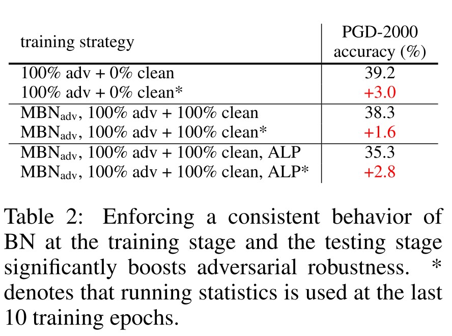
They propose a heuristic solution by applying pre-computed running statistics for model training during the last 10 epochs. As shown in Table 2, it can enhances the robustness of the resulted model.

Going deeper in adversarial training

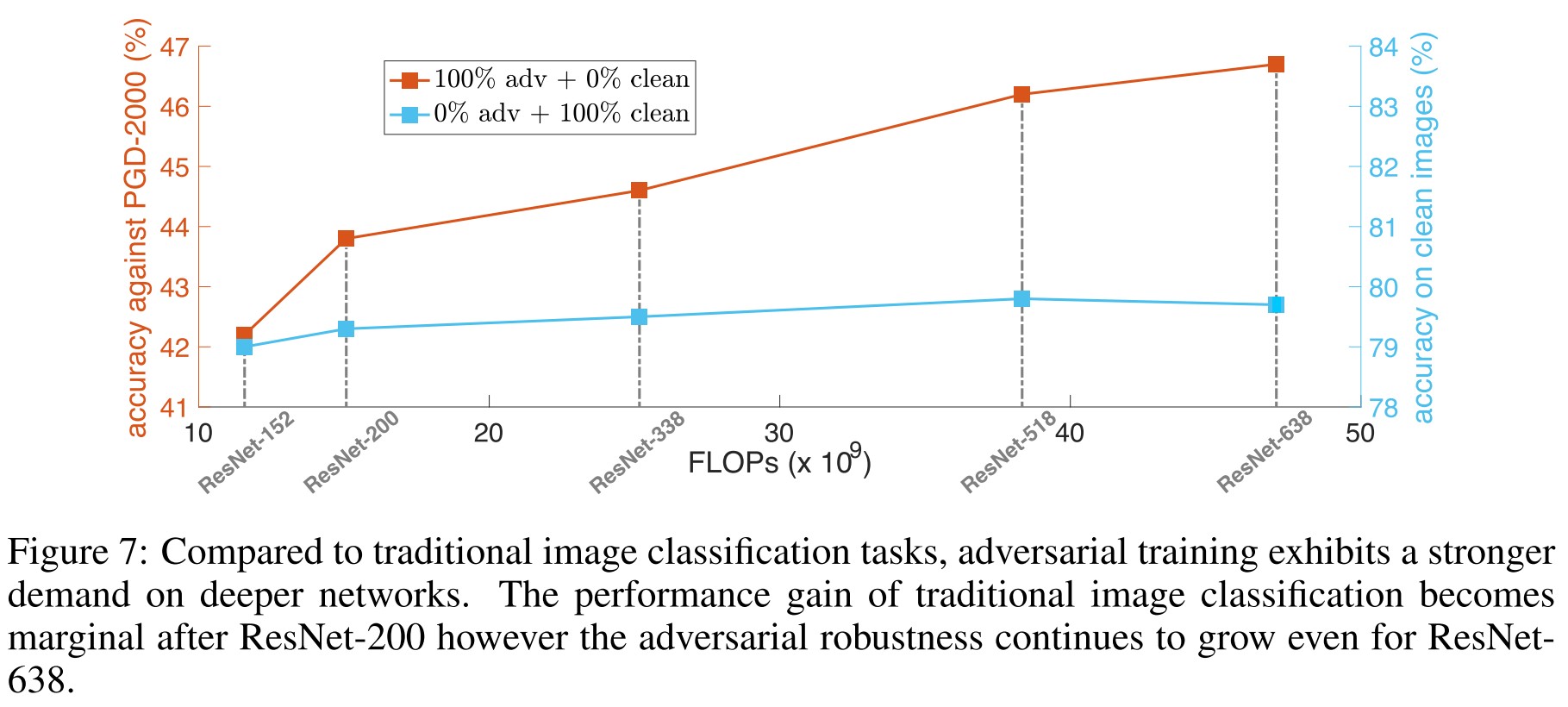
In particular, we apply the heuristic policy in Section 4.3 to mitigate the possible effects brought by BN. We observe that adversarial learning task exhibits a strong “thirst” on deeper networks to obtain stronger robustness

Inspirations

It's an interesting work. Although the claim that clean images and adversarial images may be drawn from different distributions is not solid theoretically enough, the empirical observations indeed show that a separated process of clean images and adversarial images in Batch Normalization layers results better robustness accuracy.

I think there may be a more solid explanation for this phenomenon. If the clean images and adversarial images are truly distributionally different, the heuristic solution that seems to still treat them as from the same distribution should not work that better.

Empirically, they also show that a deeper network shows a better robustness accuracy although not always better standard accuracy. This is countering the engineering wish for adversarial training.

Overfitting in adversarially robust deep learning - 2020

Code: https://github.com/locuslab/robust_overfitting

Leslie Rice, Eric Wong, J. Zico Kolter. Overfitting in adversarially robust deep learning. arXiv preprint 2020 arXiv:2002.11569

We find that overfitting to the training set does in fact harm robust performance to a very large degree in adversarially robust training across multiple datasets (SVHN, CIFAR-10, CIFAR-100, and ImageNet) and perturbation models ($l_{\infty}$ and $l_2$).

The performance gains of virtually all recent algorithmic improvements upon adversarial training can be matched by simply using early stopping.

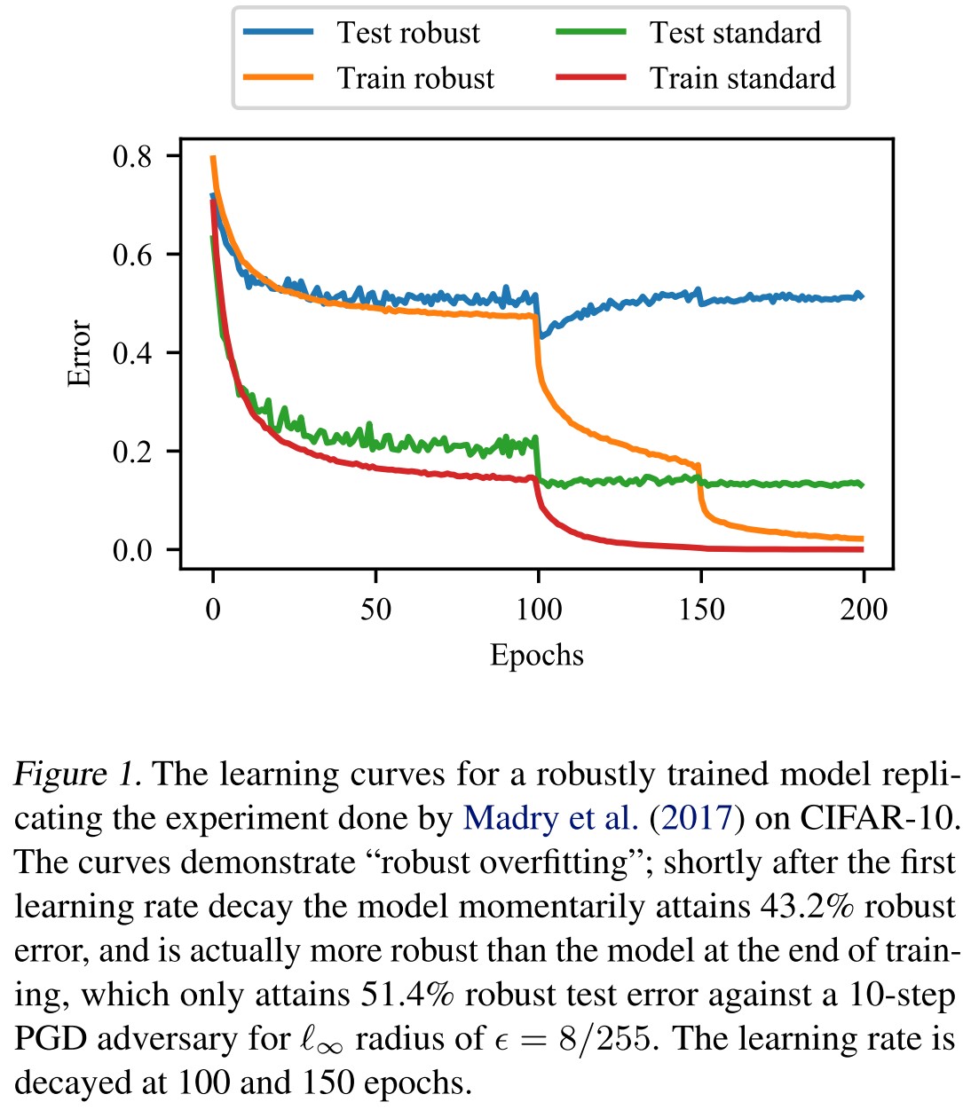
They empirically discover that overfitting hurts the adversarial training unlike the traditional deep learning that the training error can be reduced to zero with no detrimental effects on the generalization performance.

I think this explains why a larger model is better and why more data are favored in adversarial training.

Robust overfitting

Unlike the standard setting of deep networks, overfitting for adversarially robust training can result in worse test set performance.

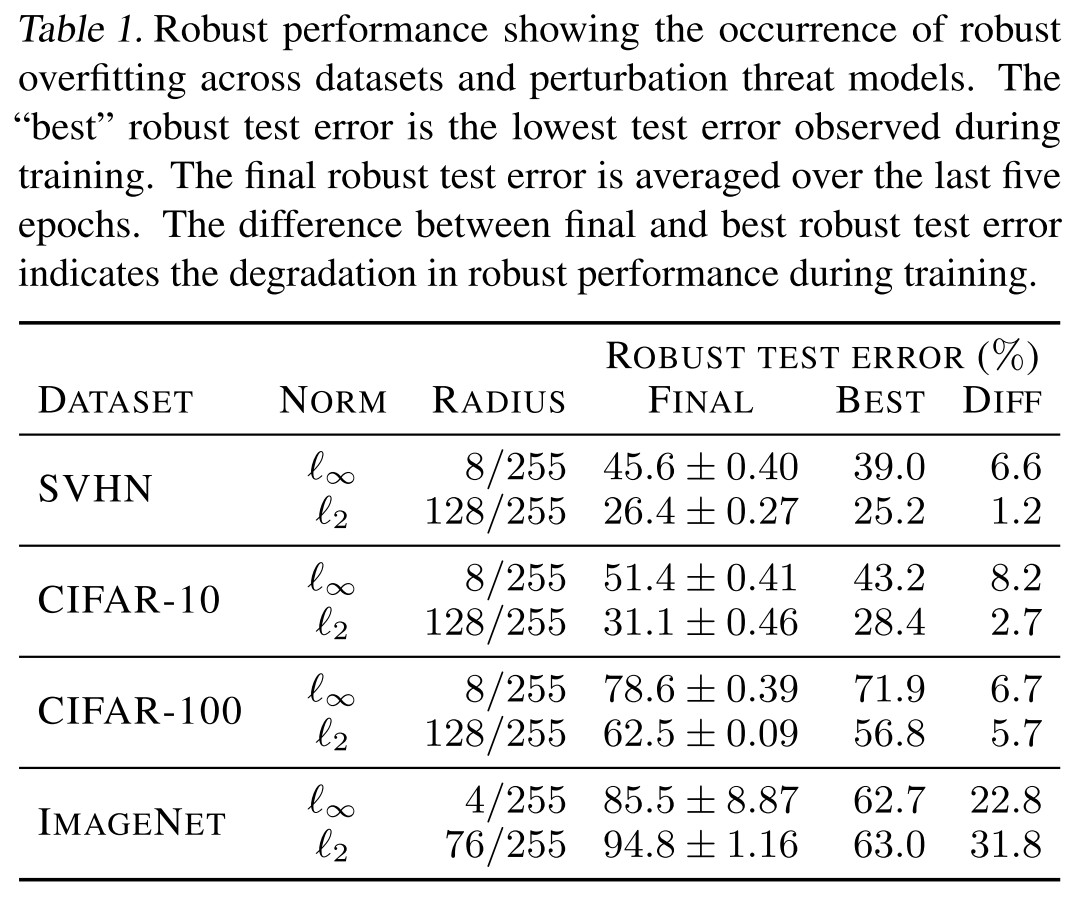
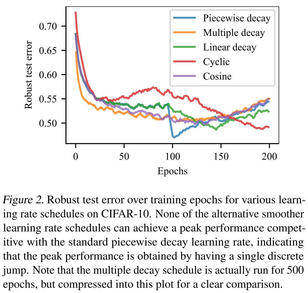
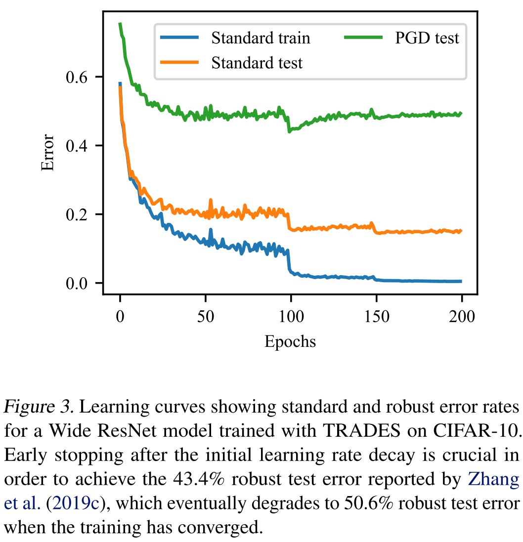
As shown in Table 1, Figure 2 and Figure 3, robust overfitting occurs in different datasets, different learning schedules and different adversarial training methods (TRADES).

Surprisingly, when we early stop vanilla PGD-based adversarial training, selecting the model checkpoint with the best performance on the test set, we find that PGD-based adversarial training performs just as well as more recent algorithmic approaches such as TRADES.

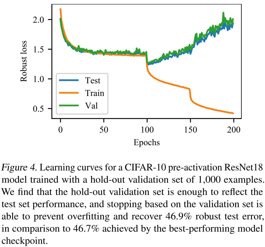
Instead, we find that it is still possible to recover the best test performance achieved during training with a true hold-out validation set.

Reconciling double descent curves

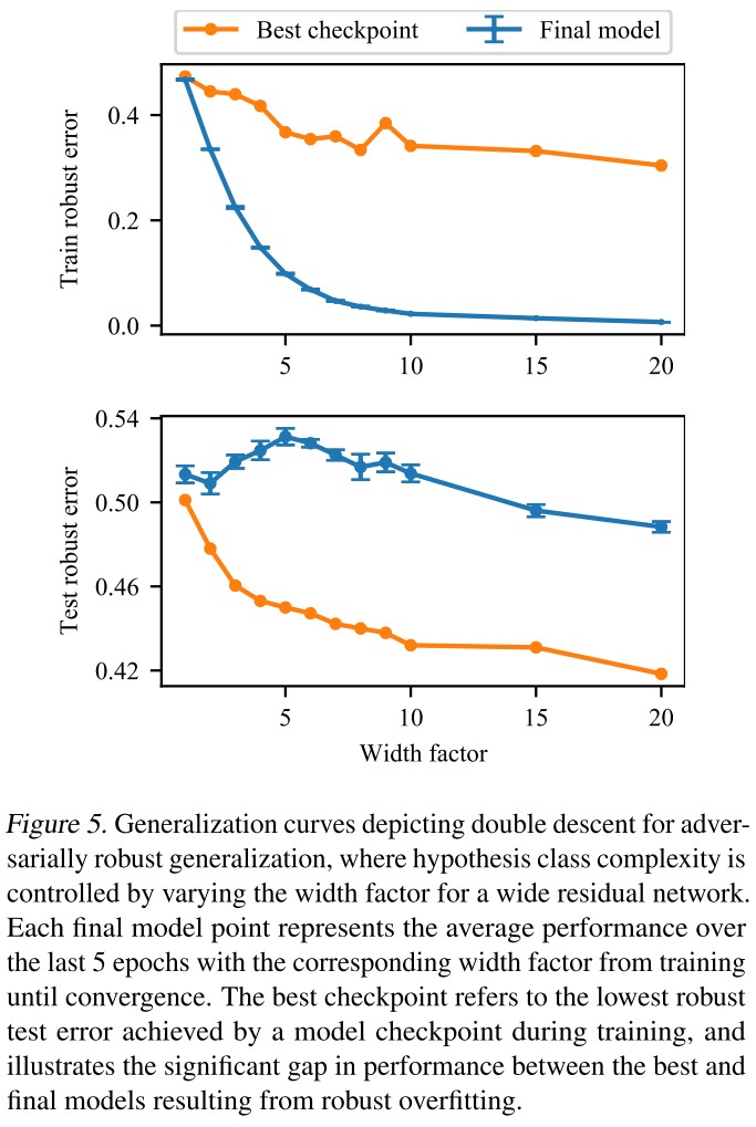
In Figure 5, we see that no matter how large the model architecture is, robust overfitting still results in a significant gap between the best and final robust test performance.

However, we also see that adversarially robust training still produces the double descent generalization curve, as the robust test performance increases and then decreases again with architecture size, suggesting that the double descent and robust overfitting are separate phenomenon

Larger architecture sizes are still beneficial for adversarially robust training despite robust overfitting.

Alternative methods to prevent robust overfitting

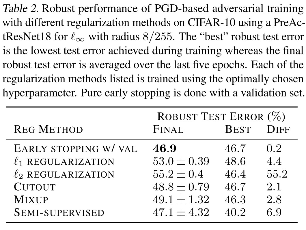
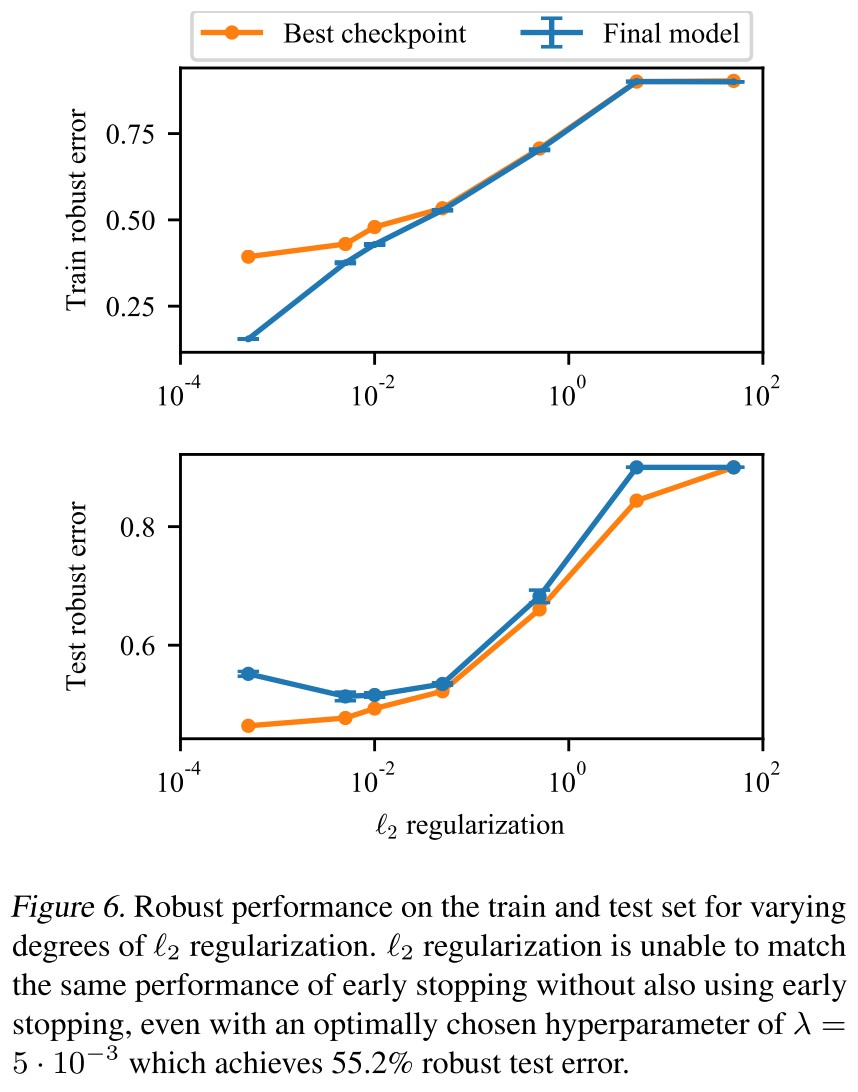
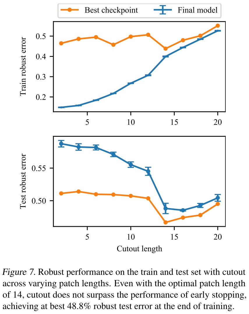
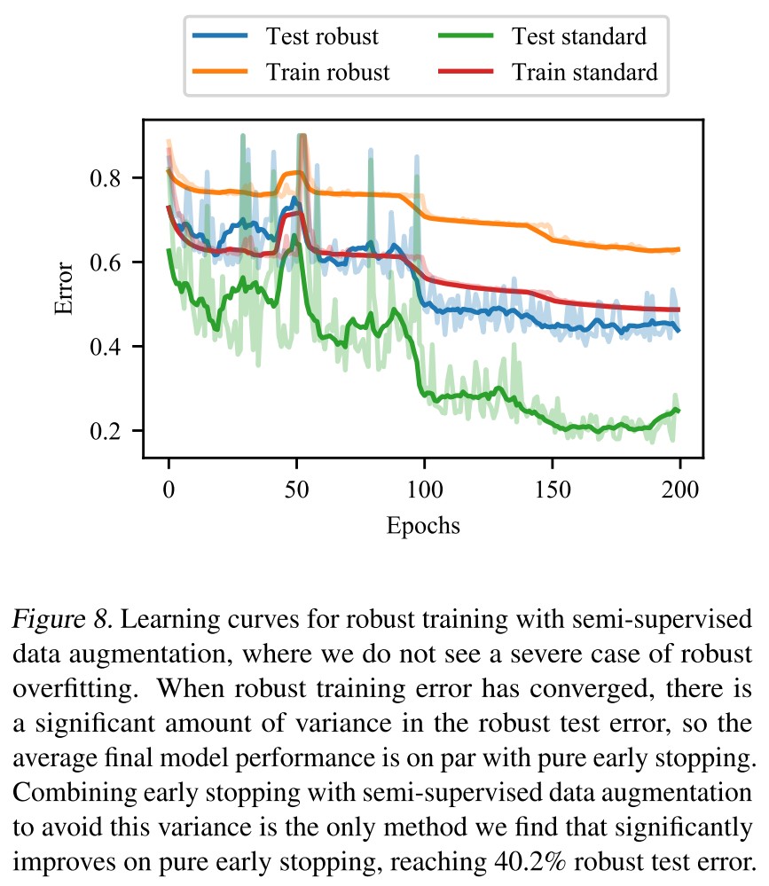
Ultimately find that no technique performs as well in isolation as early stopping.

Inspirations

This observations provide explanation for the conclusion that for adversarial training, a larger model and more data are favored.

The U-curve of the adversarial training deserves further investigation and deeper explanation.

Interpretation

A Spectral View of Adversarially Robust Features - NIPS 2018

Shivam Garg, Vatsal Sharan, Brian Hu Zhang, Gregory Valiant. A Spectral View of Adversarially Robust Features. NIPS 2018. arXiv:1811.06609

We establish strong connections between adversarially robust features and a natural spectral property of the geometry of the dataset and metric of interest.

The goal of this work is to provide a new perspective on robustness to adversarial examples, by investigating the simpler objective of finding adversarially robust features.

Robustness to Adversarial Perturbations

Definition 1 A function $f:\R^d\to \R$ is said to be $(\varepsilon,\delta,\gamma)$ robust to adversarial perturbations for a distribution $D$ over $\R^d$ with respect to a distance metric $dist:\R^d\times \R^d\to\R$ if, for a point $X$ drawn according to $D$, the probability that there exists $X^{'}$ such that $dist(x,x^{'})\le\varepsilon$ and $|f(x)-f(x^{'})|\ge \delta$, is bounded by $\gamma$, formally,

They define robustness in the form of probability. If a function is less likely to change outputs to perturbations, then the function is more robust according to the definition.

For a $(\varepsilon,1,\gamma)$ robust binary classifier $f$, the adversarial perturbations of magnitude $\varepsilon$ will make the classification accuracy of $f$ suffer at most $\gamma$.

Their approach is to map each datapoint to a feature value (or set of values) that is robust to perturbations of the points in the dataset.

Given a dataset $X$ consisting of $n$ points in $\R^d$, we desire a function $F$ that takes as input $X$, and outputs a vector $F(X)\in\R^n$; such a function $F$ is robust for a dataset $X$ if, for all $X^{'}$ obtained by perturbing points in $X$, $F(X)$ and $F(X^{'})$ are close.

They intend to build an adversarial filter that filters out adversarial perturbations to a certain extent.

For a set of all datasets consisting of $n$ points in $\R^d$, denoted as $\mathcal{X}$ and a distance metric on datasets, i.e. $dist(X,X^{'})=\max_{i\in[n]}dist(x_i,x_i^{'}),x_i\in X, x^{'}_i\in X^{'}$, they redefined the robustness of a function as follows:

Definition 2 A function $F:\mathcal{X}\to\R^n$ is said to be $(\epsilon,\delta)$ robust to adversarial perturbations for a dataset $X$ with respect to a distance metric $dist(\cdot,\cdot)$, if for all datasets $X^{'}$ (perturbed from $X$) such that $dist(X,X^{'})\le\epsilon$, $||F(X)-F(X^{'})||\le\delta$.

If a function $F$ is $(\epsilon,\delta)$ robust for a dataset $X$, it implies that feature values of 99% of the points in $X$ will not vary by more than $\frac{10\delta}{\sqrt{n}}$ if we were to perturb all points in $X$ by at most $\epsilon$.

For a single datapoint, the robust function $F_X(x)$ should follow two conditions

1. $F_x$ should have significant variance across points, e.g. (To make it separable.)

   $$\sum_{i}(F_X(x_i)-\Bbb{E}_{x\sim Unif(X)}[F_X(x)])^2=1$$

2. Changing the order of points in dataset $X$ should not change $F_X$, i.e. for any permutation $\sigma$

   $$\sigma:\R^n\to\R^n,F_{\sigma(X)}=\sigma(F_X)$$

Spectral Graph Theory

Let $G=(V(G),E(G))$ be an undirected, possibly weighted graph, where $V(G)=\{1,\dots,n\}$.

Let $A=(a_{ij})$ be the adjacency matrix of $G$, and $D$ be the diagonal matrix whose $i$th diagonal entry is the sum of edge weights incident to vertex $i$.

The matrix $L=D-A$ is called the Laplacian matrix of the graph $G$.

The normalized/scaled Lapalacian matrix is defined by

The quadratic form, and hence the eigenvalues and eigenvectors, of $L$ carry a great deal of information about $G$, e.g. for any $v\in\R^n$, we have

Apart from the apparent eigenvalue of $0$ and the eigenvector of $v_1=(1,1,\dots,1)$ that satisfies $v^\top L v=0$. The second eigenvector is the solution to the minimization problem

This characterization of the second eigenvector sounds similar in spirit to a characterization of a robust feature.

Robust features

They then construct a connection between the robust features and the second eigenvalue of the Laplacian matrix of a graph.

For a dataset $X=\{x_1,\dots,x_n\}$, define $G(X)$ to be the graph whose nodes correspond to points in $X$. If $dist(x_i,x_j)\le T$, there is an edge between nodes $x_i$ and $x_j$.

Let $L(X)$ be the (un-normalized) Laplacoan of $G(X)$ and let $\lambda_k(X)$ and $v_k(X)$ be the $k$th smallest eigenvalue and its corresponding unit eigenvector.

Then, they define $F_X(x_i)=v_2(X)_i$, i.e. the component of $v_2(X)$ corresponding to $x_i$, thus $F_X$ satisfies the requirement 1.

For a fixed $\epsilon>0$, they then define the graph $G^{+}(X)$ to be the graph with the same nodes as $G(X)$, but the edge threshold is $T+2\epsilon$. Similarly, they define $G^{-}(X)$ with the threshold $T-2\epsilon$. Other notations follow the same meanings.

Theorem 1 For any pair of datasets $X$ and $X^{'}$, such that $dist(X,X^{'})\le\epsilon$, the function $F:\mathcal{X}_n\to\R^n$ obtained using the second eigenvector of the Laplacian as defined above satisifies

Theorem 1 essentially guarantees that the features, as defined above, are robust up to sign-flip, as long as the eigengap between the second and third eigenvalues is large, and the second eigenvalue does not change significantly if we slightly perturb the distance threshold used to determine whether an edge exists in the graph in question.

They further extend the Theorem 1.

They define the $i$th feature vector for a dataset $X$ as $F_X^i=v_{i+1}(X)$. This gives a set of $k$ diverse feature vectors $\{F_X^1,F_X^2,\dots,F_X^k\}$.

Let $F_X(x)=(F_X^1(x),F_X^2(x),\dots,F_X^k(x))^\top$ be a $k$-dimensional column vector denoting the feature values for point $x\in X$.

Theorem 2 For any pair of datasets $X$ and $X^{'}$, such that $dist(X,X^{'})\le\epsilon$, there exists a $k\times k$ invertible matrix $M$, such that the features $F_X$ and $F_X^{'}$ as defined above satisfy

Inspirations

This paper has its novelty in constructing the dataset as a graph by the distances between data points, but fails to convey the idea canonically. I didn't finish it.

Basically, it proposes to use the column cutting of the eigenvectors of the connected graph of the datasets to get robust features and leaving the problem to calculate the connecting threshold for edges.

It sounds great academically, but the computation is too heavy to work through the whole dataset and get the thresholded adjacency matrix of the corresponding graph, then computing the eigenvectors....

I believe separating robust features is a promising approach, but a more efficient method is required for its prosper.