Optimism in the Face of Adversity

By LI Haoyang 2020.12.17 | 2021.1.9

Content

Optimism in the Face of Adversity - 2020

Guillermo Ortiz-Jimenez, Apostolos Modas, Seyed-Mohsen Moosavi-Dezfooli, Pascal Frossard. Optimism in the Face of Adversity: Understanding and Improving Deep Learning through Adversarial Robustness. arXiv preprint 2020. arXiv:2010.09624

This is a review. Most of these notes are directly taken from the original paper.

In this article, we provide an in-depth review of the field of adversarial robustness in deep learning, and give a self contained introduction to its main notions.

The goal of this article is to provide readers with a set of new perspectives to understand deep learning, and to supply them with intuitive tools and insights on how to use adversarial robustness to improve it.

Geometric View of Adversarial Robustness

Classification Framework

A deep neural network classifier can be described as a function $f_{\theta}:\mathcal{X}\to\mathcal{Y}$, parametrized by a set of variables $\theta\in\mathcal{W}$, which maps any input vector $x\in\mathcal{X}$ to a label $y\in\mathcal{Y}$.

Assume the weight space $\mathcal{W}=\R^M$, the input space $\mathcal{X}=\R^D$ and the output space $\mathcal{Y}=\{1,\dots,C\}$, the role of a classifier is to partition the whole input space into a set of regions with a classification label.

The decision boundary $\mathcal{B}$ of the classifier can then be defined as the set of points that lies at the intersection of two classification regions with different labels.

Given a data distribution $\mathcal{D}$ over pairs $(x,y)$, the goal of a learning algorithm is to find a classifier $f_{\theta}$ that maps any input $x$ to a label $y$, such that its expected risk on $\mathcal{D}$ is minimized, i.e.

where $\mathcal{L}(x,y;\theta)$ defines a suitable loss function between the output of a network $f_{\theta}(x)$ and the true class label $y$.

In practice, we only have a set of training samples $\{(x^{(i)},y^{(i)})\}_{i=1}^N\sim\mathcal{D}^N$. The problem is usually approximated with empirical risk minimization, i.e.

The difference between the expected risk and empirical risk attained by a classifier is known as the generalization gap of a classifier.

Modern feed-forward neural networks are formed by the composition of multiple layers where the output $z_t\in\R^{D_k}$ of layer $t$ depends only on the output of the previous layers, i.e.

where $h_t:\R^{D_{t-1}}\times\cdots\times\R^{D_0}\times\R^{M_t}\to\R^{D_t}$ can be any general differentiable or subdifferentiable mapping parametrized by some weights $\theta_t\in\R^{M_t}$.

It normally consists of the combination of linear operators (e.g., convolutions) and pointwise non-linearities (e.g., rectified linear units (ReLU)).

In classification settings, the entries of the output of the last layer $z_{L}\in\R^{D_L}$ with $D_{L}=C$ are generally referred to as logits.

Logits are normally mapped to a set of probabilities $p_{\theta}(x)\in[0,1]^C$ using a softmax operator, i.e.

and the predicted class of a neural network classifier is the index of the highest estimated probability

In fact, for most neural networks used in practice, a closed-form analysis of their properties, such as the analytical characterization of their classification regions, is not possible with our current mathematical tools.

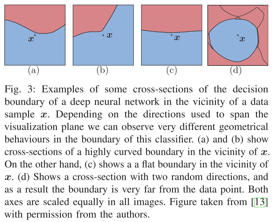
A useful way to study the properties of the decision boundary of a neural network is to visualize its cross-section with some two-dimensional plane.

Given two orthonormal vectors $u_1,u_2\in\Bbb{S}^{D-1}$, such that $u_1\perp u_2$, and a data sample $x$, we can visualize the decision boundary of a neural network $f_{\theta}$ in the vicinity of $x$ by plotting

for some specific values of $\alpha_1$ and $\alpha_2$. These cross-sections varies a lot depending on the choice of $u_1$ and $u_2$.

Besides, a notable feature of most neural networks trained on high-dimensional datasets is that, in most random cross-sections, the decision boundary appears relatively far from any typical data sample, as shown in Figure 3(d).

This can be made more rigorous if one studies the robustness of a neural network to additive random noise, i.e. the probability that a given data sample $x$ perturbed by a random vector $v\sim\mathcal{N}(0,\sigma^2I)$ is classified differently

Indeed, for most neural networks used in practice one needs to add noise with a very large variance $\sigma^2$ to fool a classifier [6].

A similarity that suggests that, despite their complex structure, neural networks create simple decision boundaries in the vicinity of data samples.

Adversarial Robustness

Surprisingly, for virtually any $x$ and $f_{\theta}$ we can always find some adversarial perturbations, which suggests that there always exist some directions for which the decision boundary of a neural network is very close to a given data sample.

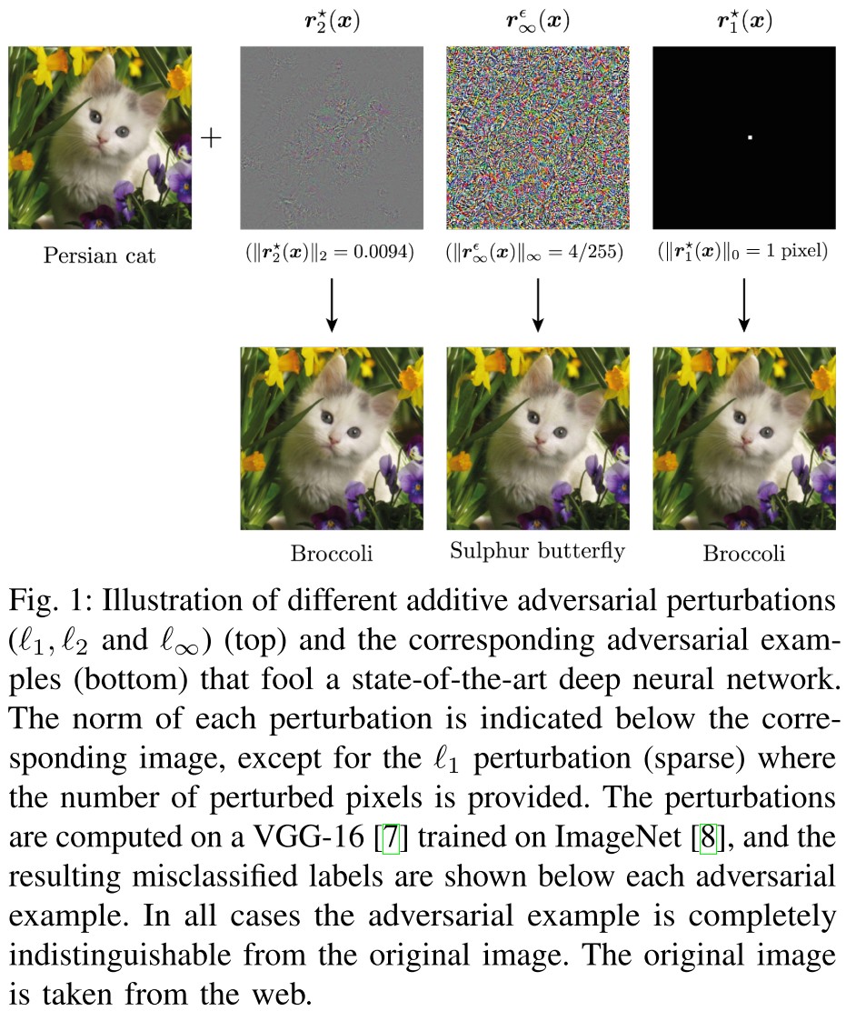
An adversarial perturbation $r(x)\in\R^D$ is defined as the solution to the following optimization problem

where $Q(r)$ represents a general objective function and $\mathcal{C}$ denotes a general set of constraints that characterize the perturbations. The perturbed samples $x+r(x)$ is referred to as adversarial examples.

Different objective and constraints lead to different adversarial examples:

• minimal $\ell_p$ adversarial perturbations $r^{*}_{p}(x)$

  $$Q(r)=||r||_p=\left(\sum_{k=1}^D([r]_k)^p\right)^{1/p}\\ \mathcal{C}=\empty$$

• $\epsilon$-constrained adversarial perturbations $r_p^{\epsilon}(x)$

  $$Q(r)=-\mathcal{L}(x+r,y;\theta)\\ \mathcal{C}=\{r\in\R^D:||r||_p\le\epsilon\}$$

• Adversarial examples have also been defined using other notions of distance2, such as geodesics in a data manifold [31]–[33], perceptibility metrics [34]–[37], Wasserstein distances [38], [39] or discrete settings [40], [41]

In the adversarial robustness literature, the algorithms that try to solve (8) are typically referred to as adversarial attacks.

Hence, most attacks only obtain an approximate solution to this problem. Surprisingly though, such approximate solutions are usually easy to find using first-order optimization methods [27]–[30].

The adversarial robustness $\rho(f_{\theta})$ of a classifier can be defined as the worst-case accuracy of a neural network subject to some adversarial perturbation, i.e.

In particular, the value of $\epsilon$ – more generally, the size of the constraint set $\mathcal{C}$ in (8) – reflects the strength of the attacker, and, in combination with the choice of metric, e.g., $\ell_p$-norm, determines the threat model of an adversary.

Measure by attack gives an upper bound of adversarial robustness, i.e. the adversarial robustness cannot be higher than it.

One can also measure robustness of a neural network as the average distance of any data sample to the decision boundary of a network, i.e.

In this geometric formulation, robustness becomes purely a property of the classifier and it is agnostic to the type of algorithm used to craft adversarial perturbations.

Still, one can verify the robustness of a classifier by checking if a safe distance exists between its decision boundaries and all data samples. That is, a classifier is certifiably $\epsilon$-robust (in an $\ell_p$-sense) if it always outputs a constant label in an $\ell_p$ ball of radius around any typical data sample.

Measure by distance to the boundary is attack agnostic and gives a lower bound of adversarial robustness, i.e. the adversarial robustness is at least it.

Adversarial training takes the attack process into the objective, i.e.

but solving it introduces much more complexity in the training.

Alternatively, there exist multiple constructive methods that try to improve robustness by maximizing (12) or (13). These algorithms are generally known as adversarial defenses.

In fact, adversarial training [27], [29], [30], a method that augments/replaces the training data with adversarial examples crafted during training, is up to this date one of the most effective adversarial defense methods.

Nevertheless, its greater computational cost – sometimes up to fifty times higher than standard training – makes it impractical for many large-scale applications.

Adversarial training, i.e. (14) is the best defense method approved in literature. But it's computationally super expensive.

Moreover, it has empirically been shown that performing adversarial training to improve the robustness to a certain type of perturbations, e.g., $r_{\infty}^{\epsilon}(x)$ does not improve robustness to other types of attacks, $r_1(x)$ [48], making the system vulnerable to other threat models [49], [50].

Adversarial training can only increase robustness in the training threat model.

Geometric Insights of Robustness

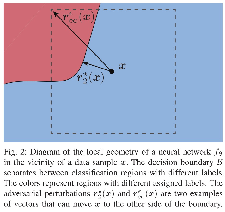
We define the local geometry of a neural network as the geometric properties of the input space of a deep classifier in an $\epsilon$-neighborhood of a data sample $x$.

The characteristics of most adversarial examples are linked to the local geometry of deep classifier by construction, i.e. they are found in the vicinity of clean examples.

For example, the success of adversarial attacks based on first-order methods to approximate (8) demonstrates that deep classifiers are relatively smooth and simple, at least in the vicinity of data samples.

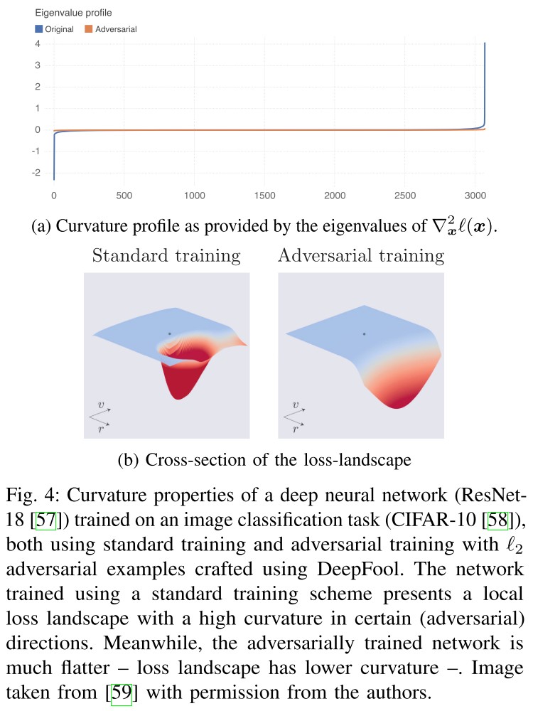
Indeed, even if popular adversarial attacks methods like FGSM [29], DeepFool [27], C&W [28], or PGD [30] are prone to get trapped in local optima in non-convex settings, their relative success demonstrates that the local geometry of deep neural networks is, in practice, approximately smooth3 and free from many irregularities (see Figure 3 and Figure 4b).

Local minimal of adversarial perturbations work well, it indicates that the decision boundary is relatively smooth and simple.

The aforementioned attacks can, therefore, be used to identify points lying exactly on the decision boundary, i.e., minimal adversarial examples.

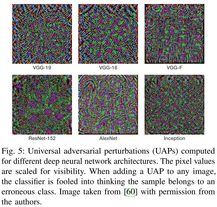
Surprisingly, these normals are very correlated among different data points, and the set of all $r_2$ perturbations of a network only spans a low-dimensional subspace of the input space [53], [54].

This explains the intriguing observation that adversarial examples transfer well between different architectures, i.e., the adversarial perturbation on a sample $x$ of a network $f_{\theta}$ is likely to fool also another network $g_{\phi}$ trained on the same dataset.

Classifiers learn the same dataset in a similar way, it brings the transferability of adversarial examples.

It naturally leads to the investigation of curvature as a central property of the local geometry of a neural network.

The loss landscape of a neural network is a function $\ell:\R^D\to\R$ that maps any input sample $x$ to $\ell(x)=\mathcal{L}(x,y;\theta)$, where $y$ is usually taken as the true label of $x$.

Using this function we can approximate the local geometry of a neural network using a second-order Taylor decomposition around $x$ and write

where $\nabla_x\ell(x)$ denotes the gradient of the loss with respect to the input, and $\nabla_x^2\ell(x)$ its second-order derivative, or Hessian.

By studying the terms in this decomposition for a trained neural network, we can discover two main things.

• $r_2^*(x)$ and $\nabla_x\ell(x)$ are very aligned in most networks, mainly due to the fact that the higher order terms in the decomposition are small. Hence the network is approximately locally linear.

• The neural networks are not completely linear as the eigen-decomposition of $\nabla_x^2\ell(x)$ demonstrates the existence of a few very curved directions in the loss landscape, as shown in Figure 4(a).

  • The predominance of zero eigenvalues in the curvature profile explains the robustness of neural networks to random noise.
  • Meanwhile, the highly curved directions explain the susceptibility of the networks to multiple adversarial attacks [54].

The minimal perturbations are very aligned with the gradients in most networks, making the attack methods based on first-order derivatives effective.

Furthermore, it has been shown [54], [55] that the principally curved directions of a deep classifier are also aligned, in the same way that the normals to the decision boundary are correlated among data points.

This explains the existence of universal adversarial perturbations, i.e.

where $0\le\delta<1$ controls the misclassification probability of the perturbations.

The connection between curvature and UAPs stems from the fact that most of the energy of UAPs is concentrated in the subspace spanned by the shared directions of high curvature.

The existence of universal adversarial perturbations indicates that the decision boundaries for most classes are curved in a similar way....

Why Geometry Matters ?

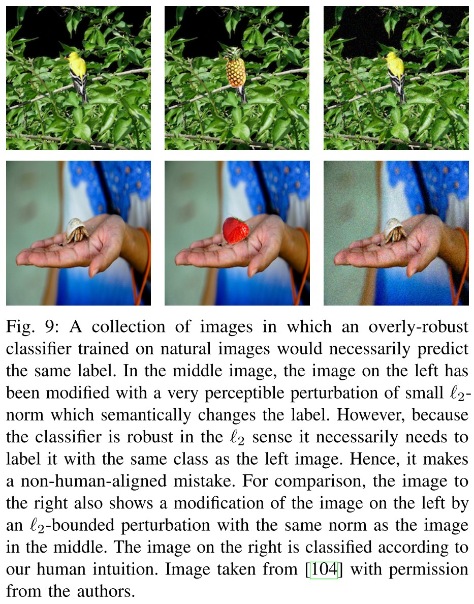
In fact, the “true” robustness is intrinsically a geometric concept, as it necessarily implies that the distance between the data points and the decision boundaries should be large.

They think that a geometrically robust model is a truly robust model, since the decision boundary is pushed away from the examples significantly.

This is a little too harsh. In practice, a model can be viewed as robust as long as in an economical profitable time, the attackers cannot find an adversarial example, or any adversarial example crafted by the attackers have a semantically different meaning from the original example.

The first – and perhaps expected – feature to notice is that adversarially trained networks seem to create boundaries that are further apart from most data samples [27]6.

However, the most interesting geometric change is the fact that the decision boundaries of adversarially trained networks exhibit a lower mean curvature than that of standard models [59] (see Figure 4a).

Adversarially trained models push the decision boundary away from data points by construction and also makes the decision boundary smoother.

Indeed, certifiable adversarial defenses, like randomized smoothing [63]–[65], also implicitly regularize curvature by averaging the decision of a classifier on randomly perturbed samples.

Making the decision boundary smoother also increases adversarial robustness.

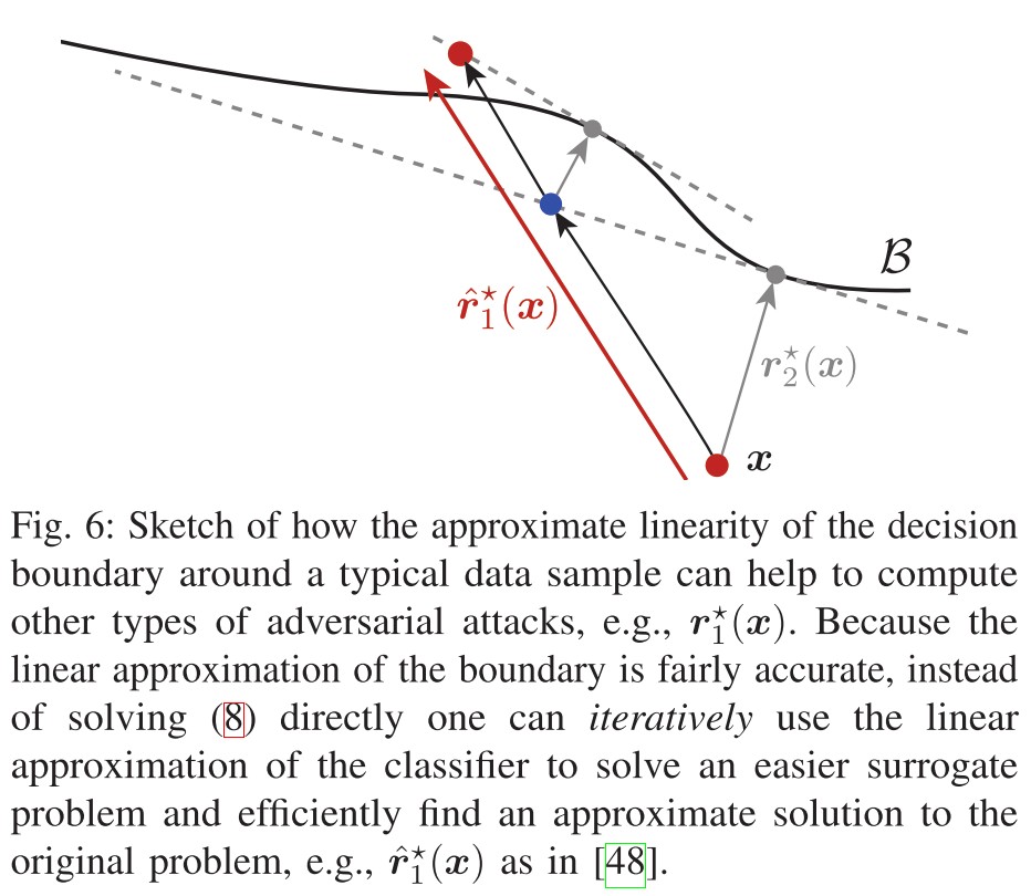
This “local flatness” property has been very important in the design of computationally efficient adversarial attacks in challenging settings like the $\ell_0$ or $\ell_1$.

The local linearity can also be exploited for better attack methods.

Discussion

Many properties of adversarial examples actually suggest that their existence is tightly linked to the way neural networks learn. Interestingly, this also means that adversarial examples may reveal important information about the inner workings of deep neural networks.

• Adversarial examples are pervasive across most applications of deep learning.
• They are very easy to compute, demonstrating the simplicity of the decision boundaries.
• They transfer across networks trained on the same dataset.
• There seem to be very strong structural similarities among adversarial examples for different data points, e.g., we can compute UAPs.

Informally speaking, one can see humans and neural networks as two classifiers with good generalization capacity that leverage very different information.

Indeed, neural networks have good test accuracy, but the existence of adversarial examples is a very strong evidence that the way neural networks generalize is by exploiting different features of the data than those humans use.

Understanding Deep Learning Through the Lens of Adversarial Robustness

Adversarial Robustness and Generalization

How is it possible that neural networks generalize so well, when their outputs are so sensitive to perturbations?

Why do most adversarial defenses, such as adversarial training, hurt performance on the clean test set?

Despite the current debate, however, there is a general consensus about the tight connection between the adversarial robustness and the generalization phenomena.

• The distribution of adversarial perturbations can predict generalization.

  In general, it has been widely observed that the distance to the decision boundary of different data samples is an important quantity for generalization.

• Adversarial examples are features.

  It's possible to train a classifier of high clean accuracy on non-robust features.

  Indeed, the fact that more robust classifiers have features which align better with our human perception is one of the main enablers of the wide range of applications of adversarial robustness beyond security.

• Adversarial robustness and accuracy trade-off.

  Following the above reasoning, one can say that the role of adversarial training – as one of the best methods to improve robustness of deep networks – is to filter out, or purify [81], the training set from non-robust features.

  If non-robust features can improve accuracy, filtering them out should naturally hurt accuracy.

  On the other hand, it seems like humans are not so susceptible to adversarial perturbations (at least the ones constructed for deep neural networks), but can still achieve good accuracy on recognition tasks, suggesting that humans do not use non-robust features.

  Human is both robust and accurate without trade-off.

  Whether there is a fundamental trade-off between adversarial robustness and accuracy, or whether the current techniques are sufficient to achieve the optimal performance in real data is still an open research debate.

Dynamics of Learning

Understanding how a neural network evolves during training is a complicated yet crucial problem that has lately attracted a lot of attention.

• Adversarial examples can be used to track the evolution of a neural network during training.

  Adversarial perturbations are linked to the features exploited by neural networks.

  In deep learning, the existence of adversarial examples seriously contends this idea, as it highlights the fact that the decision boundary of a neural network is always very close to any data sample.

  Nevertheless, the presence of this strong inductive bias in deep neural networks has recently been confirmed.

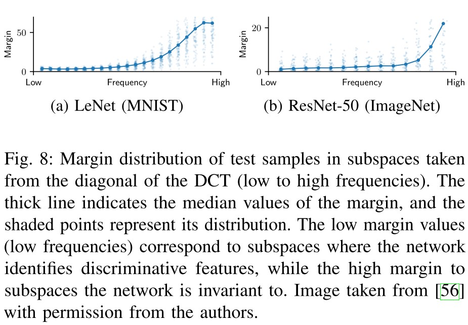
  The minimal adversarial perturbations $r^*_{2,\mathcal{S}_i}(x)$ of a neural network in a set of orthogonal subspaces $\mathcal{S}_i\sube \R^D$ can be estimated by

  $$\mathop{minimize}_{r\in\R^D}||r||_2\\ \text{subject to }f_{\theta}(x+r)\neq f_{\theta}(x),r\in\mathcal{S}_i$$

  where the norm $||r_{2,\mathcal{S}_i}^*(x)||$ gives a good estimate of the distance of the decision boundary within that subspace.

  Doing this, researchers discovered that neural networks can only create decision boundaries along those subspaces where they identify discriminative features.

  Neural networks tend to be lazy.

• Understanding adversarial training

  • Adversarially trained networks converge to solutions which are much more robust than those of standard training, and exhibit very different geometric properties.

  • Adversarially trained networks tend to show an even greater invariance than normally trained ones.

    It can be using overly-robust features, which may not be more aligned with human perception as the literature thinks.

  • Another important difference of some adversarial training schemes with regular training is their natural tendency to overfitting.

    Robust ovefitting occurs during adversarial training, which is very different from standard training that doesn't appear overfitting.

  • Related to this, another phenomenon that has complicated the evaluation of different adversarial defenses is the complex behaviour of adversarial training when trained using different adversarial attacks.

    Different attacks bring different performances. The role of attacks in adversarial training is not clarified.

• Importance of regularization

  In this sense, methods that proposed to regularize curvature [59], [61], [62], smoothness [65], [113], or gradient alignment [109] in the input space, have shown that carefully designed regularizers can drive training towards solutions with specific geometric properties in the input space, and push the decision boundary away from the data samples.

Applications of Adversarial Robustness in Machine Learning

Adversarial robustness is not only relevant to security or theoretical understanding of deep networks, it has had a significant impact on many other fields of machine learning, such as anomaly detection [117], [118], privacy [119]–[121], or fairness [122]–[127].

Interpretability of Deep Neural Networks

Interpretability and adversarial robustness are heavily related, not only because both fields make an extensive use of geometry, but also because the recently discovered connection between adversarial examples and features has opened the door to a completely new framework for interpretability.

• Interpretability and adversarial robustness.

  These methods are generally known as feature attribution methods [132]–[137] and their output is known as saliency maps.

  Connected by gradients, any attribution method that relies on the computation of $\nabla_x\ell(x)$ will necessarily be influenced by adversarial robustness.

  In particular, it has recently been proposed to use different types of image corruptions, such as deletion of objects, blurring, etc, to identify the regions of an image that can change, or preserve, the decision of a neural network.

  These are adversarial corruptions to some extent.

  Counterfactual explanations [141]–[144] extend the previous ideas to general domains, and also propose to use semantically meaningful transformations to explain the decision of a classifier.

  Most methods for obtaining counterfactual explanations can be thought as adversarial attacks, and vice-versa.

  And most interpreting methods are also vulnerable to adversarial attacks themselves.....

  Indeed, it seems that one can construct adversarial perturbations which utterly change the interpretation of almost any attribution method.

  Most interpretability methods are "adversarial attacks", and they are also vulnerable to adversarial attacks, making them unreliable.

• Robustness promotes interpretability.

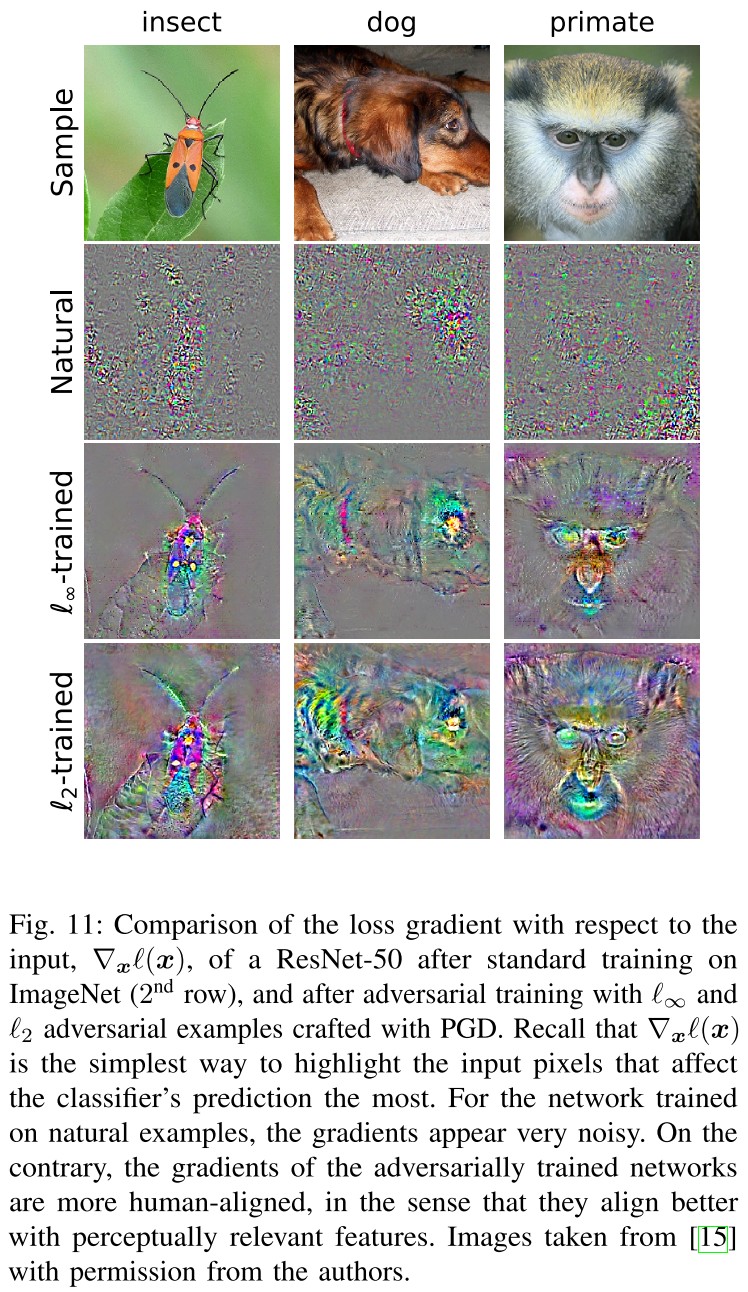
  At a high level, the robustness of a model to adversarial perturbations can be viewed as an invariance property satisfied by a classifier.

  Since human are invariant to these perturbations, therefore the model must have learned representations more aligned with human.

  Indeed, it has been shown in practice that, in contrast with standard models, the input gradients – and saliency maps – of adversarially trained networks align very well with the human perception.

  The gradient speaks for model.

  This property is universal to adversarially robust models.

Transfer Learning

Transfer learning [153], [154] refers to the common practice in deep learning by which a neural network trained on one task (source) is adapted to boost performance on another related task (target).

Here, the main assumption – which has been validated in practice [155]–[157] – is that the learned representations of the source model can be translated, or transferred, to the target model via fine-tuning.

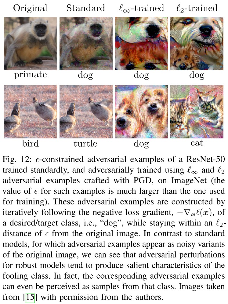
• Robustness improves transfer learning performance.

  Despite the lower standard accuracy, the transferability of a robust model is enhanced.

  A possible reason for the enhanced transferability of robust models is the observation that they have learned feature representations that correlate better with semantically meaningful features of the input images.

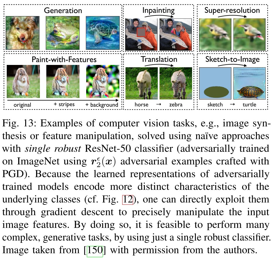
  In fact, the learned representations of adversarially trained classifiers are so powerful that they can act as an effective primitive for semantic image manipulations, unlike standard models.

  A robust model is a good semantic distance metric or loss.

• Robustness is transferable.

  Not only adversarially trained models have the ability to improve the overall performance in transfer learning tasks, but it seems that they also lead to more robust models after fine-tuning. That is, robust features are also transferable.

  One possible explanation for this phenomenon could again be the fact that adversarially trained source models act as filters of non-robust features.

  The robustness can be aligned by aligning the gradients...

Robustness to Distribution Shifts

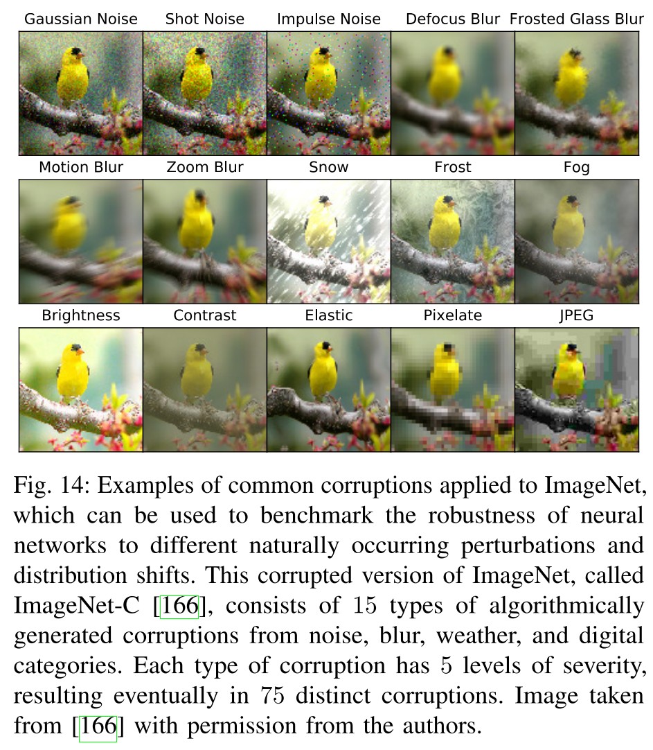
Normally trained neural networks are brittle. Not only in the adversarial sense, but also their performance suffers when their test data is slightly different than the one used for training.

In the machine learning community, the robustness to this type of general transformations is known as robustness to distribution shifts or out-of-distribution generalization.

Naturally occurring shifts can be caused due to multiple reasons such as common corruptions [166], or dataset collection biases [167] (see Figure 14).

Robustness to out of distribution is more naturally meaningful and is a line of much long history.

Adversarial robustness can act as a strong proxy for this task, allowing to compute lower bounds on the robustness of these systems, but also improve general robustness to a wide range of shifts when tuned properly.

• Adversarial robustness as a lower bound.

  Adversarial perturbation is the worst-case perturbation. The minimal additive perturbation required to move a sample $x$ to the decision boundary of a neural network given by the unit vector $v\in\Bbb{S}^{D-1}$ is

  $$r_2^v(x)=\mathop{\arg\min}_{r\in\{\alpha v:\alpha\in\R\}}||r||_2\ \text{s.t. }f_{\theta}(x+r)\neq f_{\theta}(x)$$

  and with high probability the norm of the random noise $||r_2^v(x)||_2$ required to fool the classifier is

  $$||r_2^v(x)||_2=\Theta(\sqrt{D}||r_2^*(x)||_2)$$

  meaning that improving the adversarial robustness to $r_2^*(x)$ perturbations will provably increase its robustness to random noise.

  However, for most common corruptions, we still do not have a proper mathematical characterization of the set of plausible perturbations.

• Adversarial $\ell_p$ robustness improves robustness to common corruptions

  Furthermore, adversarially trained models are more robust to perturbations that alter the high-frequency components of image data.

  Yet, although they perform better than standard models, the models that are adversarially trained using strict security budgets, e.g., large-$\epsilon$ constraints in (11), still perform poorly on the common corruption benchmarks.

• Beyond the $\ell_p$ metric

  The $\ell_p$ metric is theoretically friendly, but not accurate enough to measure the imperceptibility.

  Most of these perturbations have been studied in the context of image data and address transformations such as rotations, translations and shears [31]–[33], changes in color [34], [178], or structurally meaningful perturbations as measured by the Wasserstein metric [38], [39].

  The main problem with the above approaches is that most formulations of adversarial perturbations that do not exploit the $\ell_p$ metric, or that are not additive, are generally hard to solve.

• Adversarial robustness for confidence calibration

  The prediction of a neural network represents the probability estimated by a neural network that the input $x$ should be assigned the label $k$, but it tends to be very large.

  Nevertheless, this value is poorly calibrated in most neural networks, as it is generally very high regardless of the data sample.

  Adversarial Confidence Enhanced Training (ACET) use adversarial training to calibrate the overconfident predictions, which solves

  $$\min_{\theta}\Bbb{E}_{(x,y)\sim\mathcal{D}}[\mathcal{L}(x,y;\theta)]+\lambda\Bbb{E}_{x^\prime\not\sim\mathcal{D}_x}\left[\max_{k\in\{1,\dots,C\}}[p_{\theta}(x^\prime)]_k\right]$$

  where at every step of SGD, the $x^\prime\not\sim\mathcal{D}_x$ is acquired by a modified adversarial attack, i.e.

  $$\max_{u\in\R^D}\max_{k\in\{1,\dots,C\}}[p_{\theta}(u)]_k\\ \text{subject to }||x^\prime -u||_p\le\eta$$

  which forces the network to minimize the confidence on the sample with the largest current confidence in an $\eta$-ball around non-typical examples.

  A simple trick that improves the statistical efficiency of ACET, as it guarantees that the overconfidence of the neural network is always minimized in the worst-case sense, instead of on-average.

  Adversarial training brings significantly more uncertainty.

Other applications of adversarial robustness

In the context of anomaly detection, adversarial perturbations have been used to generate synthetic anomalous samples which do not belong to the data manifold [117], [118].

Use adversarial examples as anomaly.

In data privacy, adversarial techniques have also been exploited, for example, to identify sensitive features of a sample which can be vulnerable to attribute inference attacks [119].

Use adversarial robustness as feature filters.

However, it has also recently been argued that adversarial robust models are more vulnerable to membership inference attacks.

Adversarially trained model brings robustness and learn the dataset better, it must contain more information that may be exploited by membership inference attacks.

In the context of fairness, adversarial machine learning has recently found multiple applications [122]–[126], from the use of adversarial training to favour invariance towards racially-, or genderly-, biased features [122]; to the formulation of different notions of fairness, such as the right to an equally robust machine learning prediction [127].

Adversarial training brings some invariance for sure....

In particular, the ability of adversarial defenses to induce invariance to certain transformations of the data, and hence, learn better representations of its features, is making adversarial robustness a fundamental piece of the deep learning toolbox.

Future Research and Open Questions

Whether it is possible to obtain robust models that perform on par with standard ones in terms of accuracy, even in the strongest attack setting, is still an open problem.

How to get a robust and accurate model?

Factoring in the effect of adversarial examples in the development of new generalization bounds for deep learning is, therefore, an important line of research.

What's the generalization bounds in the presence of adversary?

Then, in relation to constructive methods, the important question of how and why do standardly trained neural networks choose, and prefer, non-robust features of a dataset remains widely open.

Why a standard model does work through the way we want?

However, obtaining models that are robust to a diverse set of naturally occurring distribution shifts stays an open problem.

Naturally adversarial examples are not well handled yet....

Also, it is important to emphasize that adversarial training is a computationally expensive procedure. For this reason, despite its ability to learn more robust representations, it is not widely adopted outside of the computer vision applications.

How to get a cheaper robust model?

Nevertheless, if we only judge the performance of robust models based on their vulnerability to certain adversarial attacks, e.g., $r_{\infty}^{\epsilon}(x)$ with a specific value of , we might overlook some other aspects of robustness beyond merely security concerns.

Using attack as the metric may overlook other benefits of the defense methods.

In general, it is important that the research on adversarial robustness should be steered towards defining novel set of benchmarks that also test the performance of adversarially robust models in other applications such as transfer learning, interpretable machine learning, and image generation.

Inspirations

This is a nice tutorial about adversarial learning, from the origin of adversarial examples to the various applications of adversarial robustness.

The following points are most interesting to me:

• How to get a robust model efficiently?
• How to improve the performance of the robust classifier on image generation?
• Is it possible that a very robust classifier is also a good generator, a good distance metric and a good object detector?
• How to get a classifier that is both accurate on clean examples and accurate on adversarial examples?
• Where does the vulnerability of a standard model come from?