Normalizing Flow

By LI Haoyang 2020.12.21 | 2020.12.30

Content

Supplementary

Change of Variables Formula

Reference: http://stla.github.io/stlapblog/posts/ChangeOfVariables.html

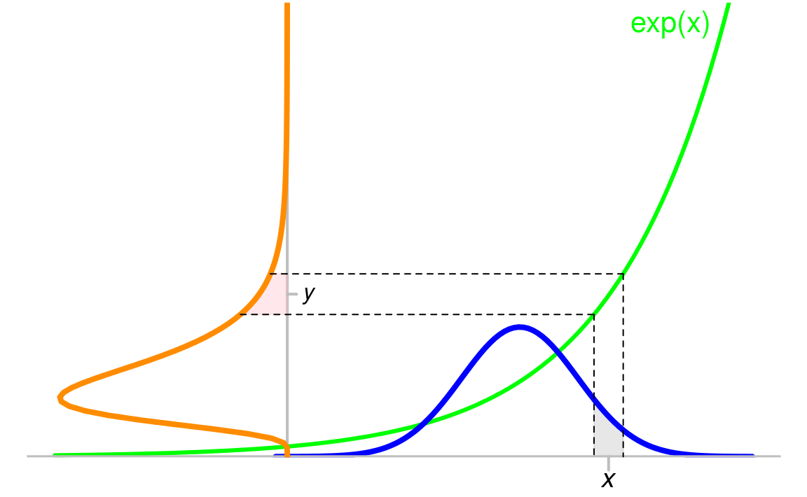
The change of variables formula refers to the calculation of the pdf of $y=g(x)$ with a given pdf of $x$.

Suppose that the pdf of $x$ is $p_x:\R^d\to\R$, and $g$ is an invertible function with the reverse as $f=g^{-1}$.

The probability that $x$ is drawn from $|dx|$ should be equal to that of $y$ drawn from $|dy|=|g^\prime(x)||dx|$ , i.e.

Therefore

Sylvester's determinant identity

Reference: https://math.stackexchange.com/questions/17831/sylvesters-determinant-identity

If $A$ and $B$ are matrices of sizes $m\times n$ and $n\times m$, then there exists

A simple proof is as follows:

Banach Fixed Point theorem

Reference: https://mathworld.wolfram.com/BanachFixedPointTheorem.html

Let $f$ be a contraction mapping from a closed subset $F$ of a Banach space $E$ into $F$. Then there exists a unique $z\in F$ such that $f(z)=z$.

A function is said to be a contraction mapping if for some $|c|<1$, there exists $|f(x)-f(y)|\le c|x-y|$, i.e. the Lipschitz constant of this function is less than 1.

Normalizing Flows: An Introduction and Review of Current Methods - TPAMI 2020

Paper: https://ieeexplore.ieee.org/document/9089305

I. Kobyzev, S. Prince and M. Brubaker, "Normalizing Flows: An Introduction and Review of Current Methods," in IEEE Transactions on Pattern Analysis and Machine Intelligence, doi: 10.1109/TPAMI.2020.2992934.

Normalizing Flows are generative models which produce tractable distributions where both sampling and density evaluation can be efficient and exact.

Generative Modeling

Generative modeling aims to model a probability distribution given examples from that distribution.

There are mainly two approaches:

• Direct analytic approaches approximate observed data with a fixed family of distributions.

  The traditional way, fit observations with priors.

• Variational approaches and expectation maximization introduce latent variables to explain the observed data.

Normalizing Flows (NF) are a family of generative models with tractable distributions where both sampling and density evaluation can be efficient and exact.

Normalizing Flow

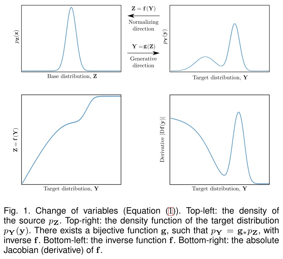
A Normalizing Flow is a transformation of a simple probability distribution (e.g., a standard normal) into a more complex distribution by a sequence of invertible and differentiable mappings.

Let $Z\in\R^D$ be a random variable with a known and tractable probability density function $p_Z:\R^D\to\R$.

Let $g$ be an invertible function, and $Y=g(Z)$.

Then, using the change of variables formula, one can compute the probability density function of the random variable $Y$:

in which:

• $f=g^{-1}$
• $Df(y)=\frac{\part f}{\part y}$ is the Jacobian of $f$
• $Dg(z)=\frac{\part g}{\part z}$ is the Jacobian of $g$

This new density function $p_Y(y)$ is called a pushforward of the density $p_Z$ by the function $g$ and denoted by $g_*p_Z$.

• Generative direction: maps a simple distribution into a more complex distribution
• Normalizing direction: maps a complex distribution back to a simple (normal) distribution

Constructing arbitrarily complicated non-linear invertible functions (bijections) can be difficult.

Let $g_1,\dots,g_N$ be a set of $N$ bijective functions and define $g=g_N\circ g_{N-1}\circ\cdots\circ g_1$ to be the composition of these functions.

Then $g$ is also bijective, with the inverse:

and the determinant of the Jacobian as:

where $Df_i(y)=\frac{\part f_i}{\part x}$ is the Jacobian of $f_i$.

The value of the $i$-th intermediate flow is denoted as

hence $x_N=y$.

Thus, a set of nonlinear bijective functions can be composed to construct successively more complicated functions.

Basically, the idea of normalizing flow is to chain a series of bijective mapping constructed using neural networks to map the given samples to a normal distribution, then the reverse can serve as a sampling function.

Formal Construction of Normalizing Flow

Definition 1. If $(\mathcal{Z},\Sigma_{\mathcal{Z}})$, $(\mathcal{Y},\Sigma_{\mathcal{Y}})$ are measurable spaces, $g$ is a measurable mapping between them, and $\mu$ is a measure on $\mathcal{Z}$, then one can define a measure on $\mathcal{Y}$, called the pushforward measure and denoted by $g_*\mu$, by the formula

The data we want to learn can be understood as a sample from a measured "data" space $(\mathcal{Y},\Sigma_{\mathcal{Y}},\upsilon)$.

To learn the data, one can introduce a simpler measured space $(\mathcal{Z},\Sigma_{\mathcal{Z}},\mu)$ and find a function $g:\mathcal{Z}\to\mathcal{Y}$ such that $\upsilon=g_*\mu$.

This function can be interpreted as a "generator", and $\mathcal{Z}$ as a latent space.

In this survey we will assume that $\mathcal{Z}=\R^D$, all sigma-algebras are Borel, and all measures are absolutely continuous with respect to Lebesgue measure (i.e., $\mu=p_Zdz$).

Definition 2. A function $g:\R^D\to\R^D$ is called a diffeomorphism, if it is bijective, differentiable, and its inverse is differentiable as well.

The pushforward of an absolutely continuous measure $p_Z dz$ by a diffeomorphism $g$ is also absolutely continuous.

Thus the theoretical foundation of normalizing flow.

Remark 3. It is common in the normalizing flows literature to simply refer to diffeomorphisms as “bijections” even though this is formally incorrect. In general, it is not necessary that $g$ is everywhere differentiable; rather it is sufficient that it is differentiable only almost everywhere with respect to the Lebesgue measure on $\R^D$. This allows, for instance, piecewise differentiable functions to be used in the construction of $g$.

Applications

Density estimation and sampling

Assume that there is only a single flow $g$ parametrized by $\theta$, and the base measure $p_Z$ is given and parametrized by the vector $\phi$.

Given a set of data observed from some complicated distribution, $\mathcal{D}=\{y^{(i)}\}_{i=1}^M$, we can then perform likelihood-based estimation of the parameters $\Theta=(\theta,\phi)$.

The data likelihood becomes

in which

• The first term is the log likelihood of the sample under the base measure.
• The second term (the log-determinant/volume correction) accounts for the change of volume induced by the transformation of the normalizing flows.

The log changes the multiplication into addition.

During training, the parameters of the flow ($\theta$) and of the base distribution ($\phi$) are adjusted to maximize the log-likelihood.

Even though a flow must be theoretically invertible, computation of the inverse may be difficult in practice; hence, for density estimation it is common to model a flow in the normalizing direction.

Variational Inference

Consider a latent variable model $p(x)=\int p(x,y)dy$, where $x$ is an observed variable and $y$ is the latent variable.

The posterior distribution $p(y|x)$ is usually intractable in practice, therefore the estimation of parameters is done with the approximate posterior $q(y|x,\theta)$, i.e. minimizing the KL divergence

which is equivalent to maximizing the evidence lower bound

The latter can be optimized using gradient descent, which requires the computation of the gradient $\nabla_{\theta}\Bbb{E}_{q(y|x,\theta)}[h(y)]$.

One can reparametrize

with normalizing flows. Assume for a single flow $g$ parametrized by $\theta$, $y=g(z|\theta)$ and the base distribution $p_Z(z)$ does not depend on $\theta$, then

and the gradient of the right hand side with respect to $\theta$ can be computed.

This approach generally to computing gradients of an expectation is often called the "reparameterization trick"

What is this $h$?

Methods

Normalizing flows should satisfy several conditions to be practical:

• Invertible; for sampling we need $g$ while for computing likelihood we need $f$.
• Sufficiently expressive to model the distribution of interest.
• Computationally efficient, both in terms of computing $f$ and $g$, but in terms of the calculation of the determinant of the Jacobian.

Elementwise Flows

A basic form of bijective non-linearity can be constructed given any bijective scalar function.

Let $h:\R\to\R$ be a scalar valued bijection.

If $x=(x_1,x_2,\dots,x_D)^\top$, then

is also a bijection.

In deep learning terminology, $h$, could be viewed as an "activation function"

Linear Flows

Linear mappings can express correlation between dimensions.

where $A\in\R^{D\times D}$ and $b\in\R^D$ are parameters. This function is invertible if $A$ is an invertible matrix.

The expressiveness of linear flows is limited. The determinant of the Jacobian is $\det(A)$, which can be computed in $\mathcal{O}(D^3)$. For computational efficiency, we can restrict the form of $A$.

• Diagonal

  If $A$ is diagonal with nonzero diagonal entries, then its inverse can be computed in linear time and its determinant is the product of the diagonal entries.

  But the diagonal matrix yields an elementwise transformation, which cannot express correlation between dimensions.

• Triangular

  The determinant of a triangular matrix is the product of its diagonal, which is much more efficient.

  Inversion is relatively inexpensive requiring a single pass of back-substitution costing $\mathcal{O}(D^2)$ operations.

• Permutation and Orthogonal

  The expressiveness of triangular transformations is sensitive to the ordering of dimensions. Reordering the dimensions can be done easily using a permutation matrix which has an absolute determinant of 1.

  The inverse and absolute determinant of an orthogonal matrix are both trivial to compute, which is efficient.

• Factorizations

  Kingma and Dhariwal [2018] proposed using the LU factorization:

  $$g(x)=PLUx+b$$

  where $L$ is lower triangular with ones on the diagonal, $U$ is upper triangular with non-zero diagonal entries, and $P$ is a permutation matrix.

  The determinant is the product of the diagonal entries of U which can be computed in $\mathcal{O}(D)$.

  The inverse of the function g can be computed using two passes of backward substitution in $\mathcal{O}(D^2)$.

  But the discrete permutation $P$ cannot be easily optimized.

• Convolution

  Convolutions are easy to compute but their inverse and determinant are non-obvious.

  Zheng et al. [2018] used 1D convolutions (ConvFlow) and exploited the triangular structure of the resulting transform to efficiently compute the determinant.

  Hoogeboom et al. [2019a] have provided a more general solution for modelling d×d convolutions, either by stacking together masked autoregressive convolutions (referred to as Emerging Convolutions) or by exploiting the Fourier domain representation of convolution to efficiently compute inverses and determinants (referred to as Periodic Convolutions).

Planar and Radial Flows

Rezende and Mohamed [2015] introduced planar and radial flows. They are relatively simple, but their inverses aren’t easily computed.

Planar Flows

Planar flows expand and contract the distribution along certain specific directions and take the following form:

where $u,w\in\R^D$ and $b\in\R$ are parameters and $h:\R\to\R$ is a smooth non-linearity.

The Jacobian determinant for this transformation is

which can be computed in $\mathcal{O}(D)$ time.

The inversion of this flow isn’t possible in closed form and may not exist for certain choices of $h(\cdot)$ and certain parameter settings.

The term $uh(w^\top x+b)$ can be interpreted as a multilayer perceptron with a bottleneck hidden layer with a single unit [Kingma et al., 2016].

Sylvester Flows

This kind of flows replaces the scaling parameters in planar flows with matrices:

where $U,W\in\R^{D\times M}$, $b\in\R^M$ and $h:\R^M\to\R^M$ is an elementwise smooth nonlinearity, where $M\le D$ is a hyperparameter to choose, which can be interpreted as the dimension of a hidden layer.

The Jacobian determinant is

where the last equality is Sylvester's determinant identity.

This can be computationally efficient if $M$ is small.

In a neural network perspective, this is a special residual block.

Radial Flows

Radial flows instead modify the distribution around a specific point so that

where $x_0\in\R^D$ is the point around which the distribution is distorted, and $\alpha,\beta\in\R$ are parameters, $\alpha>0$.

The inverse of radial flows cannot be given in closed form but does exist under suitable constraints on the parameters.

Coupling and Autoregressive Flows

Coupling Flows

Dinh et al. [2015] introduced a coupling method to enable highly expressive transformations for flows.

Consider a disjoint partition of the input $x\in\R^D$ into two subspaces: $(x^A,x^B)\in\R^d\times\R^{D-d}$ and a bijection $h(\cdot;\theta):\R^d\to\R^d$, parametrized by $\theta$.

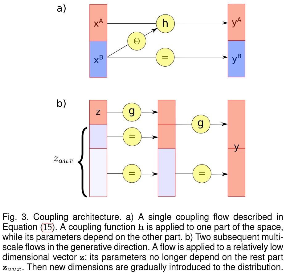
Then one can define a function $g:\R^D\to\R^D$ by the formula:

where the parameters $\theta$ are defined by any arbitrary function $\Theta(x^B)$ which only uses $x^B$ as input. It's called a conditioner.

The bijection $h$ is called a coupling function, and the resulting function $g$ is called a coupling flow.

As shown in Figure 3 (a), a coupling flow is invertible if and only if $h$ is invertible and has inverse:

Since the bijection is controlled by $x^B=y^B$, therefore one can completely reverse $y^A$ with the parameters computed from $y^B=x^B$.

The Jacobian of $g$ is a block triangular matrix where the diagonal blocks are $Dh$ and the identity matrix respectively.

Most coupling functions are applied to $x^A$ element-wise:

where each $h_i(\cdot;\theta_i):\R\to\R$ is a scalar bijection.

The power of a coupling flow resides in the ability of a conditioner $\Theta(x^B)$ to be arbitrarily complex. In practice it is usually modelled as a neural network.

As shown in Figure 3 (b), with constant conditioner, one can construct a multi-scale flow, which gradually introduces dimensions to the distribution in the generative direction.

In the normalizing direction, the dimension reduces by half after each iteration step, such that most of semantic information is retained.

For the partition of $x$:

This is often done by splitting the dimensions in half [Dinh et al., 2015], potentially after a random permutation.

Autoregressive Flows

Kingma et al. [2016] used autoregressive models as a form of normalizing flow. These are non-linear generalizations of multiplication by a triangular matrix (Section 3.2.2).

Let $h(\cdot;\theta):\R\to\R$ be a bijection parametrized by $\theta$.

An autoregressive model is a function $g:\R^D\to\R^D$, which ouputs each entry of $y=g(x)$ conditioned on the previous entries of the input:

where $x_{1:t}=(x_1,\dots,x_t)$.

Each part of $x$ is conditioned on the previous parts.

For $t=2,\dots,D$, we choose arbitrary functions $\Theta_t(\cdot)$ mapping $\R^{t-1}$ to the set of all parameters, and $\Theta_1$ is a constant. The functions $\Theta_t(\cdot)$ are called conditioners.

The Jacobian matrix of the autoregressive transformation $g$ is triangular. Each output $y_t$ only depends on $x_{1:t}$, and so the determinant is just a product of its diagonal entries:

In practice, it’s possible to efficiently compute all the entries of the direct flow.

The computation of the inverse is inherently sequential which makes it difficult to implement efficiently on modern hardware as it cannot be parallelized.

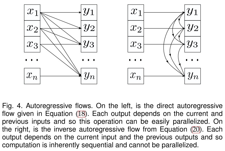
Alternatively, the inverse autoregressive flow (IAF) outputs each entry of $y$ conditioned the previous entries of $y$, i.e.

which is the same form with autoregressive flow, but the inverse of IAF can be computed relatively efficiently as shown in Figure 4.

Typically, papers model flows in the normalizing direction, i.e. from data to the base density, while IAF is a flow in generative direction.

For fast sampling, IAF is better; for fast density estimation, MAF is better.

For several autoregressive flows the universality property has been proven [Huang et al., 2018; Jaini et al., 2019a].

Informally, universality means that the flow can learn any target density to any required precision given sufficient capacity and data.

Residual Flows

Residual networks are compositions of the function of the form:

Such a function is called a residual connection, and here the residual block $F(\cdot)$ is a feed-forward neural network of any kind.

The first attempts to build a reversible network architecture based on residual connections were made in RevNets [Gomez et al., 2017] and iRevNets [Jacobsen et al., 2018].

Consider a disjoint partiton of $\R^D=\R^d\times\R^{D-d}$ denoted by $x=(x^A,x^B)$ for the input and $y=(y^A,y^B)$ for the output, and define a function:

where $F:\R^{D-d}\to\R^d$ and $G:\R^d\to\R^{D-d}$ are residual blocks. This network is invertible but computation of the Jacobian is inefficient.

A different point of view on reversible networks comes from a dynamical systems perspective via the observation that a residual connection is a discretization of a first order ordinary differential equation.

To make the residual connection $g(\cdot)$ invertible, a sufficient condition is found that

Propostion 7. A residual connection is invertible, if the Lipschitz constant of the residual block is $Lip(F)< 1$.

There is no analytically closed form for the inverse, but it can be found numerically using fixed-point iterations (which, by the Banach theorem, converge if we assume Lip(F) < 1).

The specific architecture proposed by Behrmann et al. [2019], called iResNet, uses a convolutional network for the residual block. It constrains the spectral radius of each convolutional layer in this network to be less than one.

Infinitesimal (Continuous) Flows

The residual connection can be viewed as discretizations of a first order ordinary differential equation (ODE):

where $F:\R^D\times\Theta\to\R^D$ is a function which determines the dynamic (the evolution function), $\Theta$ is a set of parameters and $\theta:\R\to\Theta$ is a parametrization.

The discretization of this quation (Euler's method) is

which is equivalent to a residual connection with a residual block $\varepsilon F(\cdot,\theta_n)$.

This similarity is marvelous.

The rest of this part is a little out of my understanding... for now.

Discussion and Open Problems

Inductive biases

No more than prior, structure and loss function.

Role of the base measure

The base measure of a normalizing flow is generally assumed to be a simple distribution (e.g., uniform or Gaussian).

Theoretically the base measure shouldn’t matter: any distribution for which a CDF can be computed, can be simulated by applying the inverse CDF to draw from the uniform distribution.

However in practice if structure is provided in the base measure, the resulting transformations may become easier to learn.

Form of diffeomorphisms

The majority of the flows explored are triangular flows (either coupling or autoregressive architectures).

A natural question to ask is: are there other ways to model diffeomorphisms which are efficient for computation? What inductive bias does the architecture impose?

Loss function

The majority of the existing flows are trained by minimization of KL-divergence between source and the target distributions (or, equivalently, with log-likelihood maximization).

However, other losses could be used which would put normalizing flows in a broader context of optimal transport theory.

Generalisation to non-Euclidean spaces

This part is out of my mathematical level.... for now.

Inspirations

The core idea of a flow is to model distribution without information loss by insuring that the model is invertible.

Most flows are designed to be invertible, but it can also be converted from a general neural networks. The following two kinds of flows are particularly interesting to me:

• Coupling flows

  It sustains the invertibility by keeping part of information unchanged.

• Invertible Residual Network

  It insures the invertibility as long as the residual block has a Lipschitz constant smaller than 1.