Invertible Residual Networks

By LI Haoyang 2020.12.1

Content

Invertible Residual Networks - ICML 2019

Code: https://github.com/jhjacobsen/invertible-resnet

Jens Behrmann, Will Grathwohl, Ricky T. Q. Chen, David Duvenaud, Jörn-Henrik Jacobsen. Invertible Residual Networks. ICML 2019. arXiv:1811.00995

We show that standard ResNet architectures can be made invertible, allowing the same model to be used for classification, density estimation, and generation.

In contrast, our approach only requires adding a simple normalization step during training, already available in standard frameworks.

They make the standard ResNet invertible by adding a simple normalization step during training.

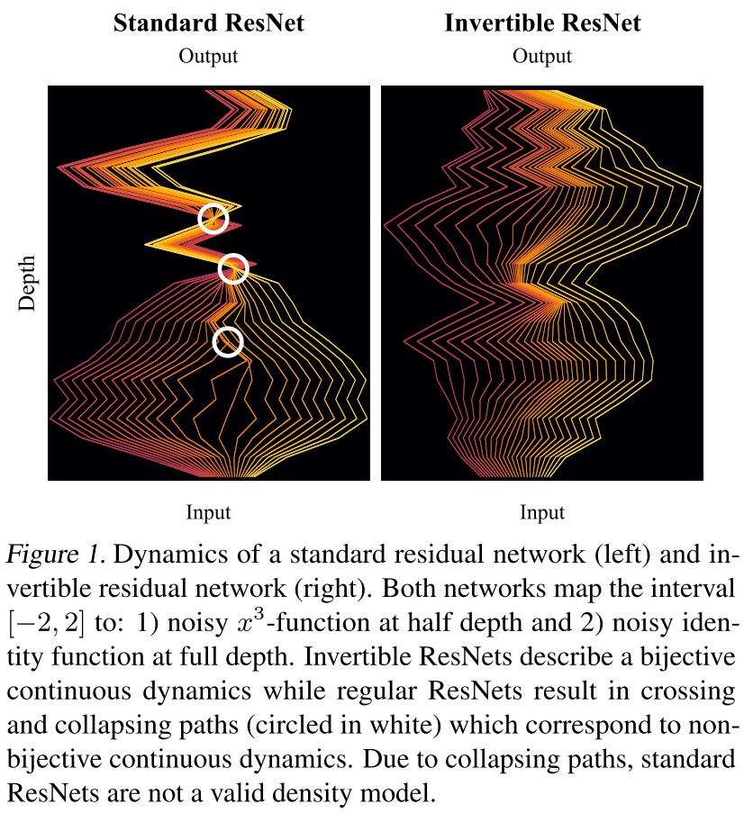
This approach allows unconstrained architectures for each residual block, while only requiring a Lipschitz constant smaller than one for each block.

Enforcing invertibility in ResNets

The architectures of ResNet are very similar to Euler's method for ODE initial value problems:

where:

• $x_t\in\R^d$ represents activations or states
• $t$ represents layer indices or time
• $h>0$ is a step size
• $g_{\theta_t}(x_t)$ is a residual block

This connection has attracted research at the intersection of deep learning and dynamical systems.

Reversely, solving the dynamics backwards in time would implement an inverse of the corresponding ResNet, i.e.

Theorem 1 (Sufficient condition for invertible ResNet). Let $F_{\theta}:\R^d\to\R^d$ with $F_{\theta}=(F_{\theta}^1\circ\cdots\circ F_{\theta}^T)$ denote a ResNet with blocks $F_{\theta}^t=I+g_{\theta_t}$. The ResNet $F_{\theta}$ is invertible if

where $Lip(g_{\theta_t})$ is the Lipschitz-constant of $g_{\theta_t}$.

Why?

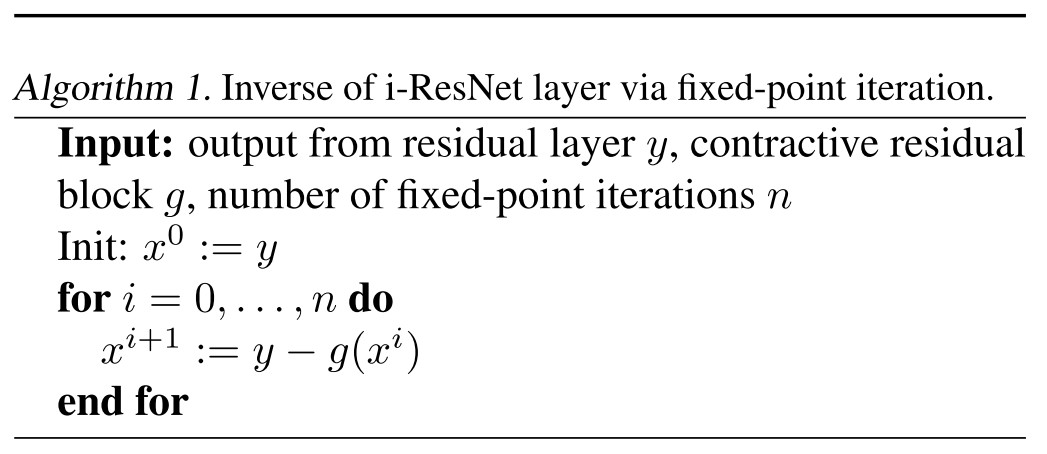
The inverse of ResNet block can be obtained through a simple fixed-point iteration, as shown in Algorithm 1.

From the Banach fixed-point theorem, there is

the convergence rate is exponential in the number of iterations $n$ if using the output $y=x+g(x)$ as the initial point, and a smaller Lipschitz constants will yield faster convergence.

If $x^0=y$, then $x^1=y-g(x^0)=y-g(y)$, and $||x^1-x^0||_2=||g(y)||_2$.

A contractive residual block also renders the residual layer bi-Lipschitz.

Lemma 2 (Lipschitz constants of Forward and Inverse). Let $F(x)=x+g(x)$ with $Lip(g)=L<1$ denote the residual layer. Then it holds

Hence by design, invertible ResNets offer stability guarantees for both their forward and inverse mapping.

As long as each block has a Lipschitz constant smaller than one, it's possible to use simple iterations to find the inverse.

Satisfying the Lipschitz constraint

They implement residual blocks as a composition of contractive nonlinearities $\phi$ (e.g. ReLU, ELU, tanh) and linear mappings.

For a network with three convolutional layers, i.e.

There is

where $||\cdot||_2$ denotes the spectral norm.

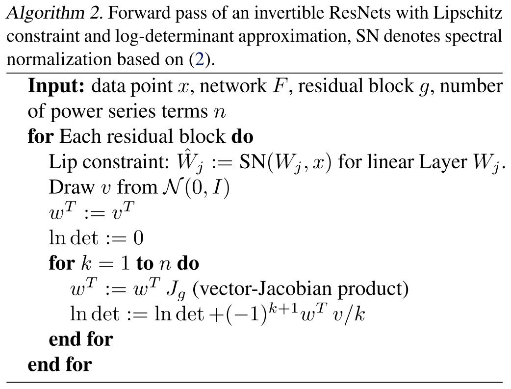
They directly estimate the spectral norm of $W_i$ by performing power-iteration using $W_i$ and $W_i^T$ , yielding an under-estimate $\tilde{\sigma}_i\le||W_i||_2$, using which they normalize the weight via

where $c<1$ is a scaling coefficient.

They show that $Lip(g)<1$ holds in all cases, since $||W_i||_2\le c$ is not guaranteed with the under-estimate $\tilde{\sigma}_i$.

Normalizing flow with i-ResNets

For data $x\in\R^d$, we can define a simple generative model by first sampling $z\sim p_z(z)$ where $z\in\R^d$ and then defining $x=\Phi(z)$ with some function $\Phi:\R^d\to\R^d$.

First map an artificial distribution into data distribution.

If $\Phi$ is invertible, define $F=\Phi^{-1}$, we can compute the likelihood of any $x$ under this model using the change of variables formula:

where $J_F(x)$ is the Jacobian of $F$ evaluated at $x$.

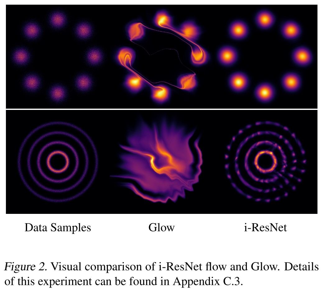
As shown in Figure 2, using i-ResNet is better than Glow.

Approximation of log-determinant

Computing $\ln|\det J_F(x)|$ naively has a time complexity of $\mathcal{O}(d^3)$, in order to scale to higher dimensions, they propose to approximate it.

The Lipschitz constrained perturbations $x+g(x)$ of the identity yield positive determinants, i.e.

and for non-singular matrix $A\in\R^{d\times d}$, there exists

Combining them, there is

Thus for $z=F(x)=(I+g)(x)$, it becomes

The trace of matrix logarithm can be expressed by a power series

which converges if $||J_g||_2<1$.

Hence, due to the Lipschitz constraint, we can compute the log-determinant via the above power series with guaranteed convergence.

Due to $Lip(g_t)<1$ for the residual block of each layer $t$, the log-determinant of gradient can be upper and lower bounded

Thus, both the number of layers T and the Lipschitz constant affect the contraction and expansion bounds of i-ResNets and must be taken into account when designing such an architecture

Algorithm

Using the power series to compute the log-determinant still has three main drawbacks:

1. Computing $tr(J_g)$ exactly costs $\mathcal{O}(d^2)$, or approximately needs $d$ evaluations of $g$ as each entry of the diagonal of the Jacobian requires the computation of a separate derivative of $g$.
2. Matrix powers $J_g^k$ are needed, requiring the knowledge of the full Jacobian.
3. The series is infinite.

To overcome 1 and 2, they use vector-Jacobian products $v^\top J_g$ and the Hutchinsons trace estimator to estimate the trace of a matrix $A\in\R^{d\times d}$ stochasticly, i.e.

where the distribution $p(v)$ needs to fulfill $\Bbb{E}[v]=0$ and $Cov(v)=I$. (A normal distribution?)

To overcome 3, they truncate the series at index $n$, i.e.

They give an error bound for this truncation.

Theorem 3 (Approximation error of Loss). Let $g$ denote the residual function and $J_g$ the Jacobian as before. Then, the error of a truncated power series at term $n$ is bounded as

Smaller Lipschitz constant, longer term and lower dimension yield a smaller error.

They also give a convergence analysis.

Theorem 4 (Convergence Rate of Gradient Approximation). Let $\theta\in\R^p$ denote the parameters of network $F$, let $g,J_g$ be as before. Further, assume bounded inputs and a Lipschitz activation function with Lipschitz derivative. Then, we obtain the convergence rate

where $c:=Lip(g)$ and $n$ the number of terms used in the power series.

In practice, only 5-10 terms must be taken to obtain a bias less than .001 bits per dimension, which is typically reported up to .01 precision (See Appendix E).

Experiments

Invertible classification

Using Algorithm 1.

We invert each residual connection using 100 iterations (to ensure convergence).

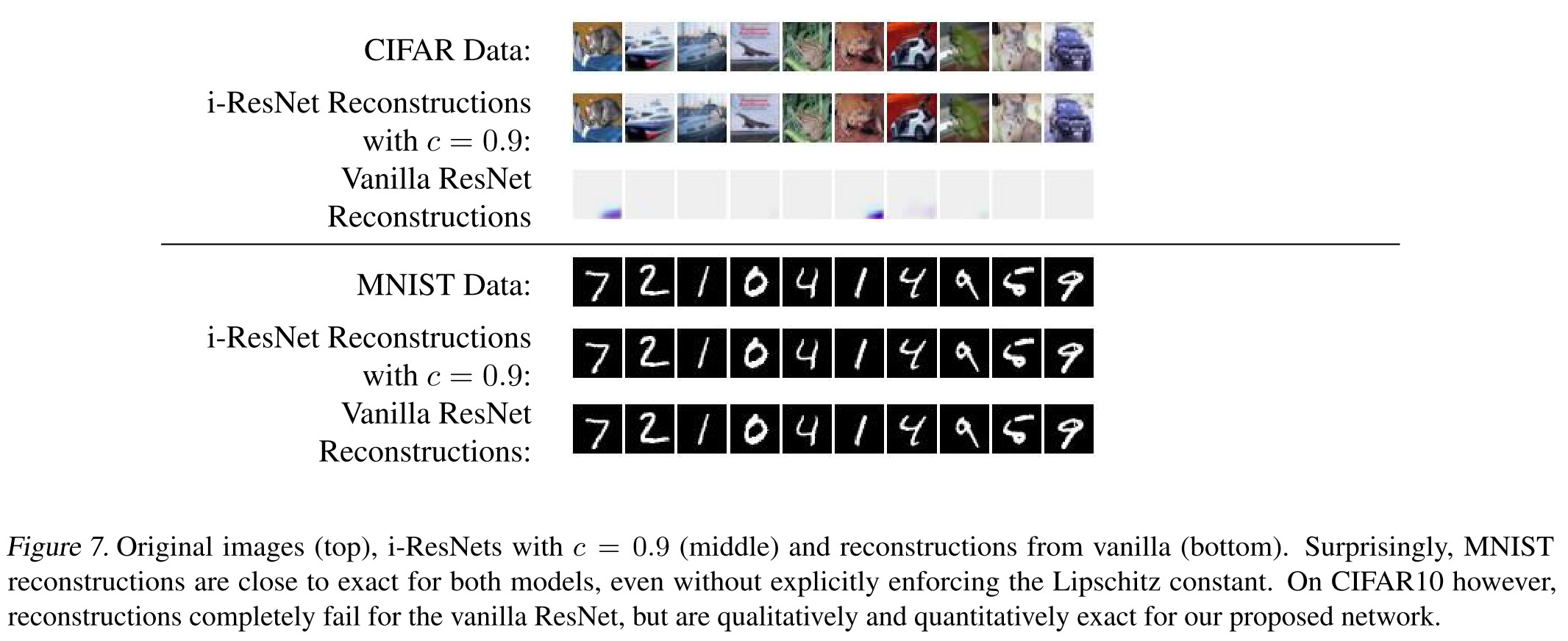
We see that i-ResNets can be inverted using this method whereas with standard ResNets this is not guaranteed (Figure 7 top). Interestingly, on MNIST we find that standard ResNets are indeed invertible after training on MNIST (Figure 7 bottom).

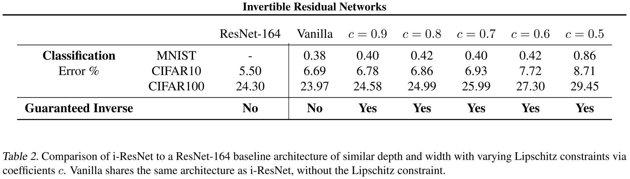
Our proposed invertible ResNets perform competitively with the baselines in terms of classification performance.

In summary, we observe that invertibility without additional constraints is unlikely, but possible, whereas it is hard to predict if networks will have this property.

Generative modeling

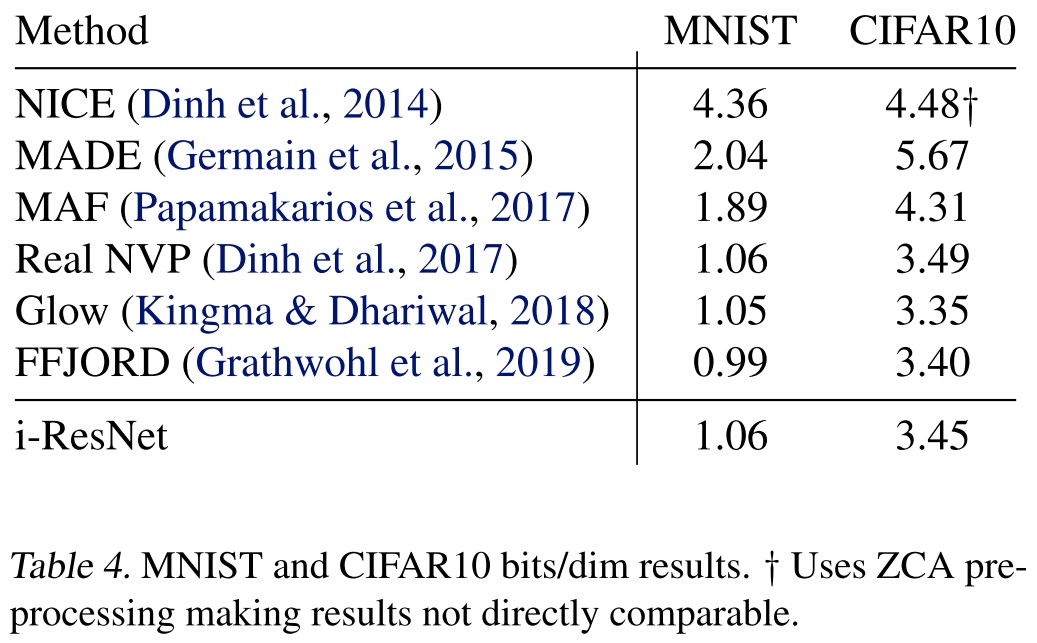
As shown in Table 4

While our models did not perform as well as Glow and FFJORD, we find it intriguing that ResNets, with very little modification, can create a generative model competitive with these highly engineered models.

Inspirations

It's just amazing that using such simple constraint can make a ResNet invertible.

Note that this network constrains the Lipschitz constant for each residual block to be smaller than one, which is similar to some technique in adversarial defense, and the ability to reconstruct images from features is also manifested in adversarially trained networks, I think there is some work that combines them.