Feature Purification : an Explanation for Adversarial Training

By LI Haoyang 2020.12.10

Content

Feature Purification: How Adversarial Training Performs Robust Deep Learning - 2020

Zeyuan Allen-Zhu, Yuanzhi Li. Feature Purification: How Adversarial Training Performs Robust Deep Learning. arXiv preprint 2020. arXiv:2005.10190

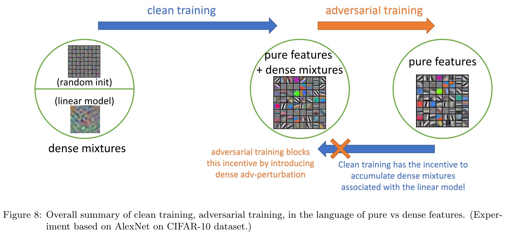
In this paper, we present a principle that we call feature purification, where we show one of the causes of the existence of adversarial examples is the accumulation of certain small dense mixtures in the hidden weights during the training process of a neural network; and more importantly, one of the goals of adversarial training is to remove such mixtures to purify hidden weights.

They study the learning process of adversarial training and propose the idea of feature purification as a principle of robust deep learning, i.e. trying to answer the following questions:

Why do adversarial examples exist when we train the neural networks using the original training data set? How can adversarial training further “robustify” the trained neural networks against these adversarial attacks?

For a simplified standard model, they prove that:

1. Training over the original data is indeed non-robust to small adversarial perturbations of some radius.
2. Adversarial training, even with an empirical perturbation algorithm such as FGM, can in fact be provably robust against any perturbations of the same radius.

They also give a complexity lower bound, showing that a model under this complexity bound cannot yield robustness regardless of training algorithms.

A similar idea like feature purification was actually adopted as a defense itself several years ago by PixelDefend, which was later breached and classified as one of gradient masking methods.

This paper seems to indicate that adversarial training also utilizes feature purification, but in a better way.

The Principle of Feature Purification

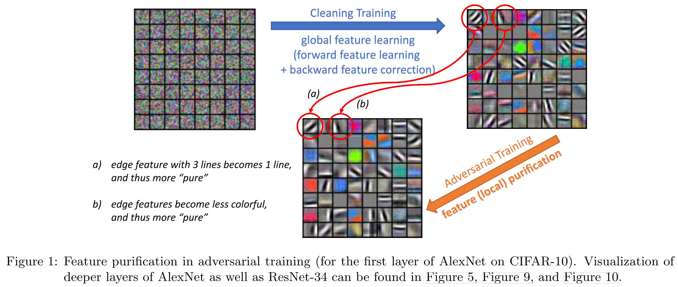
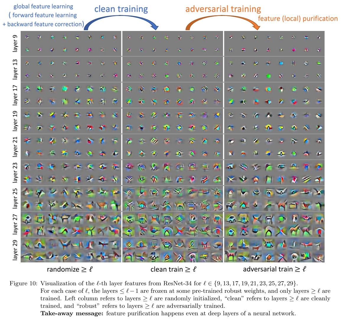
The Principle of Feature Purification During adversarial training, the neural network will neither learn new, robust features nor remove existing, non-robust features learned over the original data set. Most of the works of adversarial training is done by purifying a small part of each learned feature after clean training.

Using the following notations:

• $w_i^{(0)}$, the weight vector of the $i$-th neuron at initialization.
• $w_i$, the weight vector after clean training.
• $w_i^\prime$, the weight vector after adversarial training using $w_i$ as initialization.

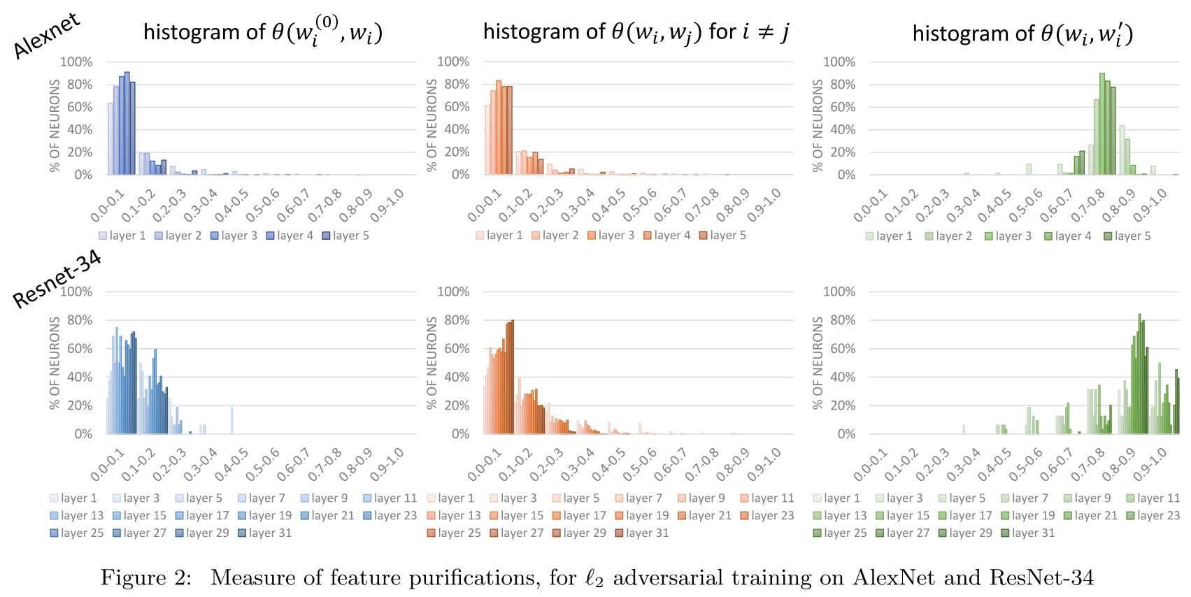
And the following provisional measure of correlation between "features":

i.e. the absolute value of cosine similarity.

They have the following claims:

• For most neurons: $\theta(w_i^{(0)},w_i),\theta(w_i^{(0)},w_i^\prime)\le c$ for a small constant $c$ (such as 0.2).
• For most neurons: $\theta(w_i,w_i^\prime)\ge C$ for a large constant $C$ (such as 0.8).
• For most pairs of different neurons: $\theta(w_i,w_j)\le c$ for a small constant $c$ (such as 0.2).

A small cosine similarity implies a large difference.

As a result, this principle implies that both clean training and adversarial training discover hidden weights $w_i,w_i^\prime$ fundamentally different from the prescribed initialization $w_i^{(0)}$.

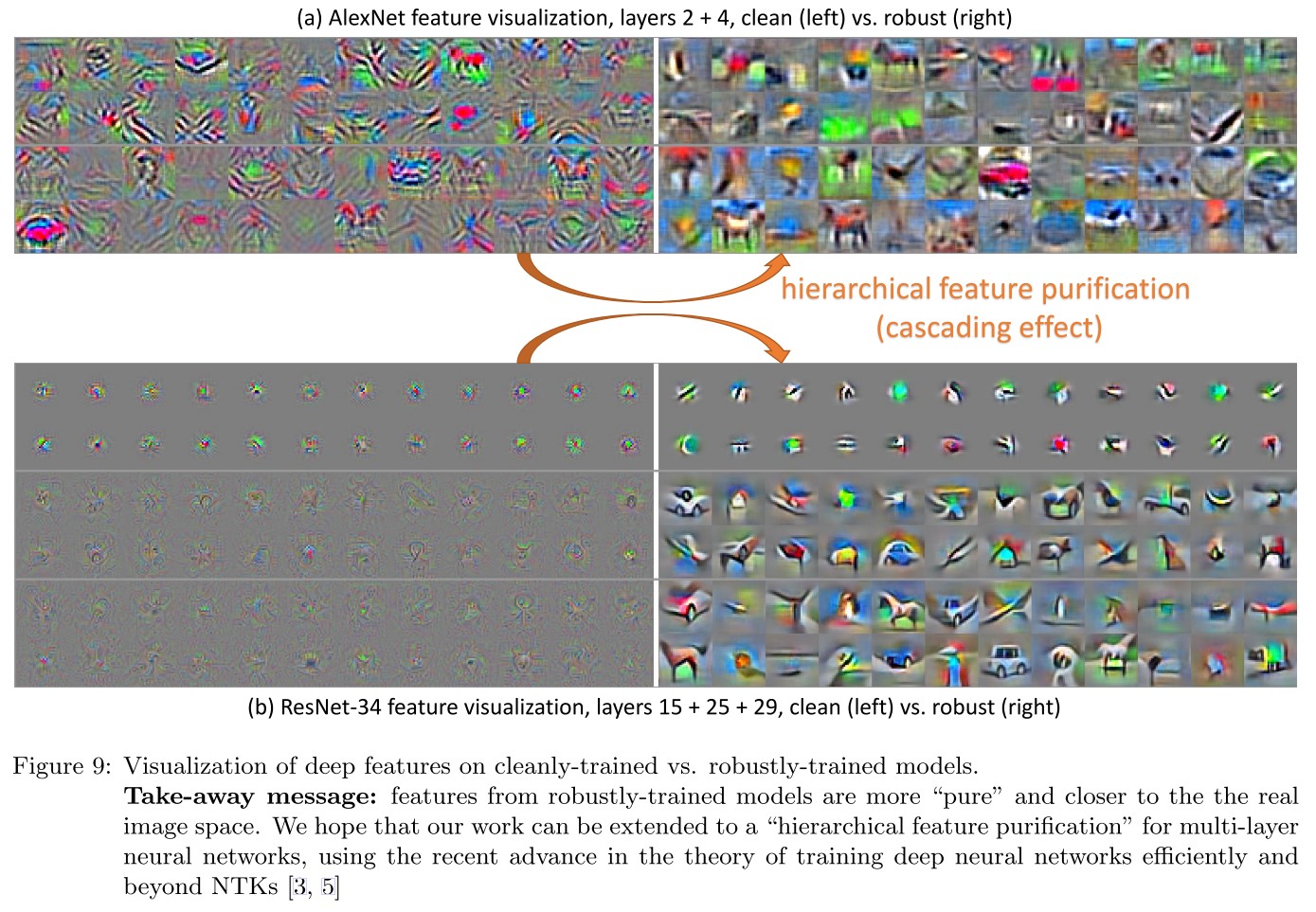
They propose that clean training already discover a big portion of the robust features while adversarial training further purifies them.

Well, two weights both differ from initialization and they are relatively similar, so it indicates that adversarial training purifies the weights....It's a little shaky.

Why clean training learns non-robust features? Which part of the features are “purified” during adversarial training?

As we shall formally discuss in Section 6.2, training algorithms such as gradient descent will, at every step, add to the current parameters a direction that maximally correlates with the labeling function on average.

They refer this part of weight that correlates with the average of training data as dense mixture. Since under natural assumptions of the data such as the sparse coding model, i.e. inputs come from sparse combinations of hidden dictionary words/vectors, such dense mixtures cannot have any high correlation with any individual, clean example, thus the network can still generalize well on the original dataset.

However, we show that these portions of the features are extremely vulnerable to small, adversarial perturbations along the “dense mixture” directions. As a result, one of the main goals of adversarial training, as we show, is to purify the neurons by removing such dense mixtures.

Moreover, in our setting, these dense mixtures in the hidden weights of the network come from the sparse coding structure of the data and the gradient descent algorithm.

They state that the cleanly trained model tends to learn an average of the training data, namely dense mixture which leads to the adversarial vulnerability.

Computational Complexity

We also prove a lower bound that, for the same sparse coding data model, even when the original data is linearly-separable, any linear classifier, any low-degree polynomial, or even the corresponding neural tangent kernel (NTK) of our studied two-layer neural network, cannot achieve meaningful robust accuracy (although they can easily achieve high clean accuracy).

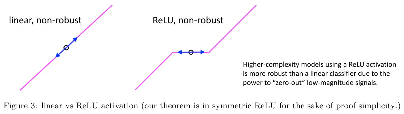
The main intuition is that low complexity models, including the neural tangent kernel, lacks the power to zero out low magnitude signals to improve model robustness, as illustrated in Figure 3 and Section 3.

Preliminaries

Notations

• $||x||$, or $||x||_2$, the $\ell_2$-norm of a vector $x$
• $||x||_p$, the $\ell_p$-norm of a vector $x$
• $\bold{M}_i$, the $i$-th column of a matrix $\bold{M}\in\R^{d\times d}$
• $||\bold{M}||_{\infty}:=\max_{i\in[d]}\sum_{j\in[d]}\bold{M}_{i,j}$, the largest sum of columns of the matrix
• $||\bold{M}||_1:=\max_{j\in[d]}\sum_{i\in[d]}\bold{M}_{i,j}$, the largest sum of rows of the matrix
• $\text{poly}(d):=\Theta(d^C)$, the degree $C$ is some not-specified constant
• $\text{sign}(x)=1$ for $x\ge 0$ and $\text{sign}(x)=-1$ for $x<0$

What is this $\Theta$?

Sparse coding model

They consider the training data $x\in\R^d$ generated from

for a dictionary $\bold{M}\in\R^{d\times D}$, where the hidden vector $z\in\R^D$ and $\xi\in\R^d$ is the noise.

They focus on $D=d$ and $\bold{M}$ is a unitary matrix.

They assume the hidden vector $z$ is "sparse", i.e. for $k\le d^{0.499}$:

Assumption 2.1 (distribution of hidden vector $z$). The coordinates of $z$ are independent, symmetric random variables, such that $|z_i|\in\{0\}\cup[\frac{1}{\sqrt{k}},1]$. Moreover,

The first condition is a regularity condition, requiring that $\Bbb{E}[||z||_2^2]=\Theta(1)$.

The second and third condition says that there is a non-trivial probability where $z_i$ attains the maximum value, and a (much) larger probability that $z$ is non-zero but has a small value.

???

Fact 2.2 Under Assumption 2.1, w.h.p., $||z||_0=\Theta(k)$ is a sparse vector.

They study the simplest binary classification problem, where the labelling function is linear over the hidden vector $z$, i.e.

For simplicity, they assume $\forall i\in[D],|w_i^*|=\Theta(1)$, i.e. all the coordinates of $z$ have relatively equal contributions.

Clean and robust error

The goal of clean training is to learn a model $f$ so that $\text{sign}(f(x))$ is as close to $y$ as possible. The classification error on the original data set is defined as:

Consider the robust error against $\ell_p$ adversarial perturbations. For a value $\tau>0$ and a norm $||\cdot||_p$, the robust error of the model $f$ is defined as

Warmup Intuitions

Linear learners are not robust

This is anti-intuitive......

A direct approach to classify the given dataset is to use a linear classifier as

and use the sign to predict label. They point out that there are two issues of this classifier:

1. When $\sigma_x$ is as large as $\Theta(1)$, such classifier cannot even classify $x$ in good accuracy, i.e.

   $$f(x)=\left<w^*,\bold{M}^\top x\right>=\left<w^*,z\right>+\left<\bold{M} w^*, \xi\right>$$

   while typically $|\left<w^*,z\right>|=O(1)$ and $\left<\bold{M} w^*,\xi^\prime\right>\sim\mathcal{N}(0,\Theta(\sigma_x^2))$ by assumption. Thus when $\sigma_x\ge \Theta(1)$, the signal is overwhelmed by the noise.

2. Even when $\sigma_x=0$, i.e. the original data is perfectly linearly classifiable, linear classifier is also not robust to small perturbations, i.e.

   one can design an adversarial perturbation $\delta=\frac{-Cu\bold{M} w^*}{||w^*||_2^2}$ for a large constant $C$ that can change the sign of the linear classifier for most inputs, given that $|\left<w^*,z\right>|=O(1)$.

   Well, I think it's DeepFool, orthogonal perturbation to the decision boundary.

   Since $||w^*||_2=\Theta(\sqrt{d})$, this linear classifier is not even robust to adversarial perturbations of $\ell_2$ norm $\Theta(\frac{1}{\sqrt{d}})$.

   It's obtained by taking the norm into the form of perturbation.

I think the first claim is weird here, the first issue states that when the noise is comparable with signal, the classifier fails, which is not the problem of linearity as far as I can see. For data with many noise, a complicated classifier also fails.

High-complexity models are more robust

Another approach is to use a higher-complexity model:

Since $\left<\bold{M}_i,x\right>=z_i+\left<\bold{M}_i,\xi\right>$, as long as the signal $z_i$ is non-zero, $|\left<\bold{M}_i,x\right>|\ge\frac{1}{2\sqrt{k}}$ with high probability.

By Fact 2.2, w.h.p. the signal $z$ is $O(k)$-sparse, i.e. there are at most $O(k)$ coordinates with the indicators to be 1, therefore this high complexity model $f(x)$ has $1-o(1)$ robust accuracy against any adversarial perturbation of $\ell_2$ radius $o(\frac{1}{\sqrt{k}})$.

How ???

Learning robust classifier using neural network

Their goal is to show that a two-layer neural networks can learn a robust function $f(x)$ after adversarial training, such as

in which:

• $ReLU(y)=\max\{y,0\}$
• $b\approx\frac{1}{2\sqrt{k}}$

In this paper, we present a theorem stating that adversarial training of a (wlog. symmetric) two-layer neural network can indeed recover a neural network of this form.

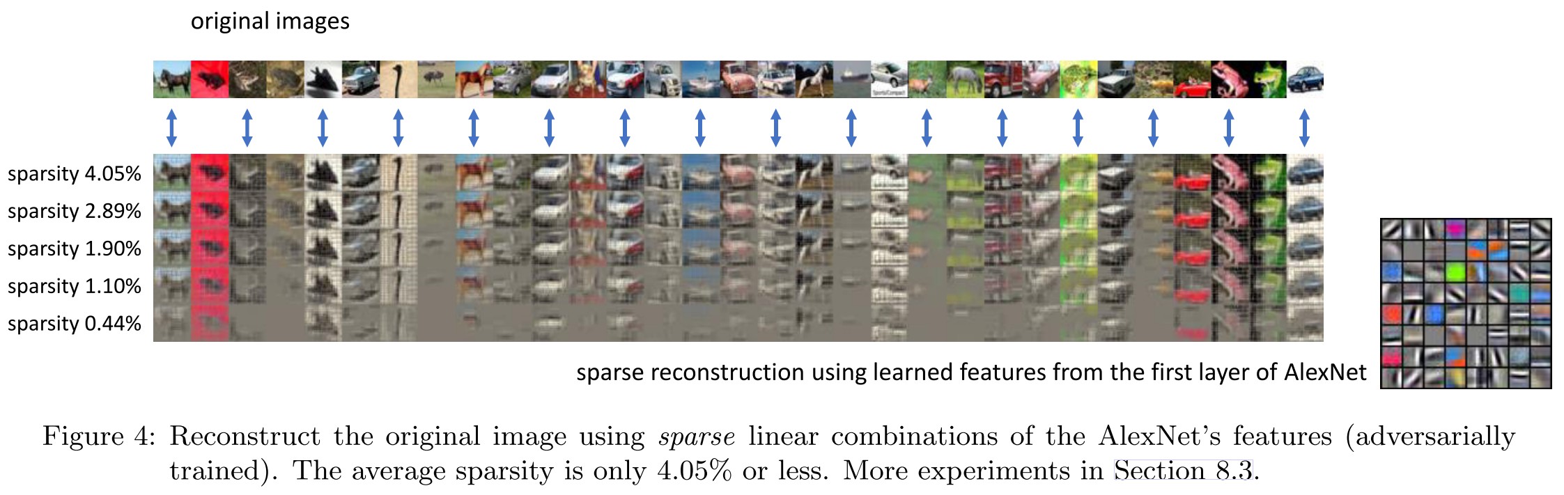
In other words, after adversarial training, the features learned by the hidden layer of a neural network can indeed form a basis (namely, $M_1,\dots,M_d$) of the input $x$ where the coefficients are sparse.

It learns a set of basises ! Are they orthogonal ? If so, then it's connected back to Parseval Network and Lipschitz Regularization.

Learner Network and Adversarial Training

They consider a simple, two layer symmetric neural network with ReLU activation, i.e.

where $f(x)=-f(-x)$, and

• $w_i\in\R^d$, the hidden weight (feature) of the $i$-th neuron
• $b_i>0$, the negative bias
• $\rho_i\sim\mathcal{N}(0,\sigma_p^2)$ is a smoothing of the original ReLU, also known as pre-activation noise; equivalently with $\widetilde{ReLU}=\Bbb{E}_{\rho}ReLU(x+\rho)$.

They use $\rho$ to denote $(\rho_i)_{i\in[m]}$.

They fix $a_i=1$ throughout the training for simplicity.

They use $w_i^{(t)}$ to denote the hidden weights at time $t$, and $f_t(w;x,\rho)$ to denote the network at iteration $t$, i.e.

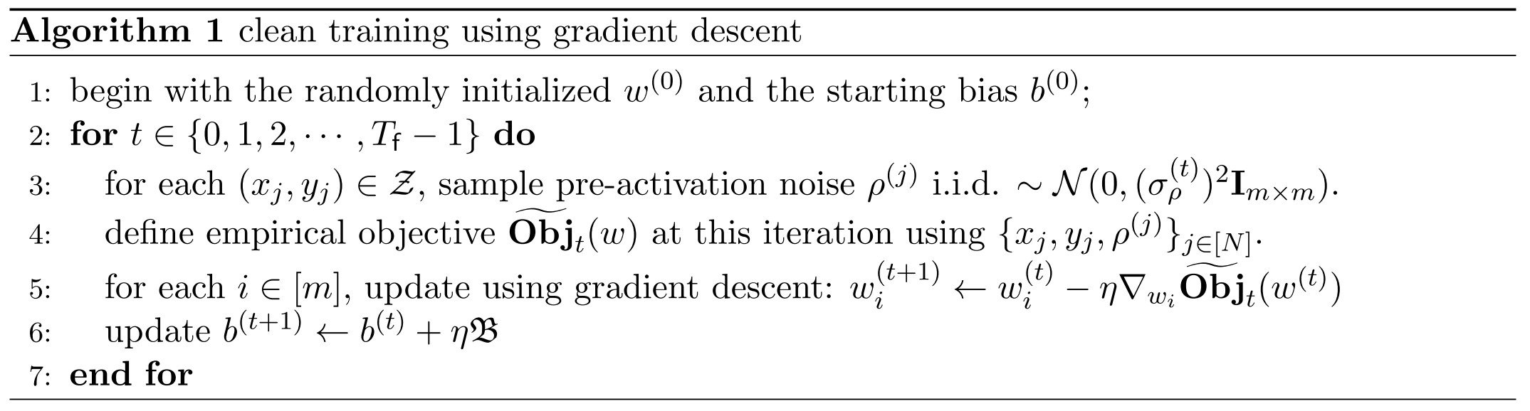
Given a training set $\mathcal{Z}=\{x_j,y_j\}_{j\in[N]}$ together with one sample of pre-activation noise $\rho^{(j)}$ for each $(x_j,y_j)$, they define:

1. $\bold{Loss}_t(w;x,y,\rho):=\log(1+e^{-yf_t(w;x,\rho)})$
2. $\bold{Loss}_t(w):=\Bbb{E}_{x,y=y(x),\rho}[\bold{Loss}_t(w;x,y,\rho)]$
3. $\widetilde{\bold{Loss}}_t(w):=\frac{1}{N}\sum_{j\in[N]}[\bold{Loss}_t(w;x_j,y_j,\rho^{(j)})]$
4. $\bold{Obj}_t(w):=\bold{Loss}_t(w)+\lambda\sum_{i\in[m]}\bold{Reg}(w_i)$
5. $\widetilde{\bold{Obj}}_t(w):=\widetilde{\bold{Loss}}_t(w)+\lambda\sum_{i\in[m]}\bold{Reg}(w_i)$

The first one is the standard logistic loss, the second one is the population risk and the third one is the empirical risk.

They consider a strong regularier:

and a fixed $\lambda$:

for simplicity.

Definition 4.1 In our case, the (clean, population) classification error at iteration $t$ is

We also introduce a notation (the logistic gradient)

and observe

What is this $\Omega$ ???

Clean Training

Details seems redundant, so it's omitted.

Adversarial Training

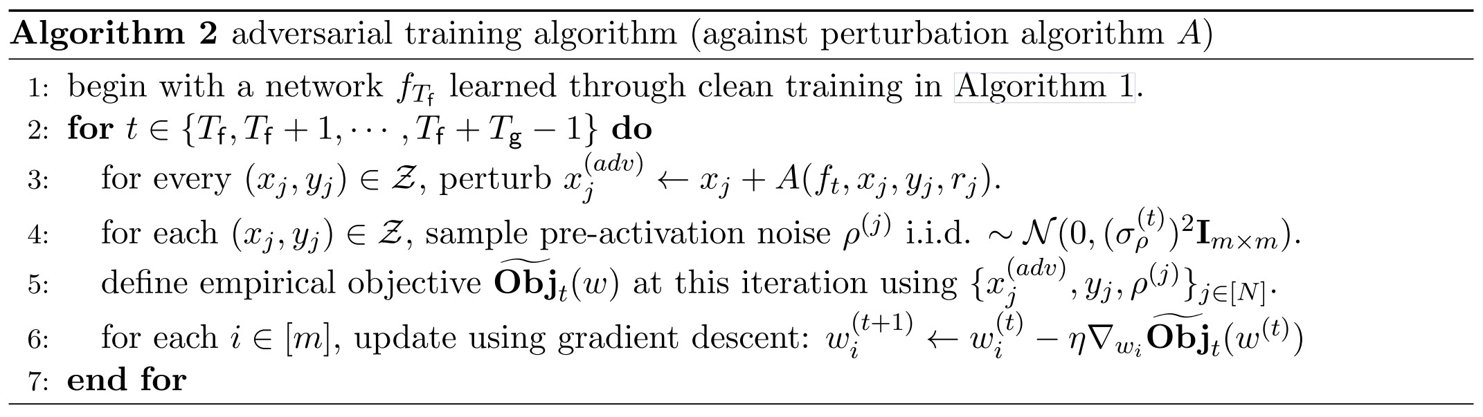
Definition 4.2. An (adversarial) perturbation algorithm $A$ (a.k.a. attacker) maps the current network $f$ (which includes hidden weights $\{w_i\}$, output weights $\{a_i\}$, bias $\{b_i\}$ and smoothing parameter $\sigma_p$), an input $x$, a label $y$, and some internal random string $r$, to $\R^d$ satisfying

for some $\ell_p$ norm. We say $A$ is an $\ell_2$ perturbation algorithm of radius $\tau$ if $p=2$, and $\ell_{\infty}$ perturbation algorithm of radius $\tau$ if $p=\infty$.

For simplicity, they assume $A$ satisfies for fixed $f,y,r$, either $||A(f,x,y,r)||_p\le\frac{1}{\text{poly}(d)}$, or $A(f,x,y,r)$ is a $\text{poly}(d)$-Lipschitz continuous function in $x$.

The FGM attack satisfies the above properties, defined as

where $||\cdot||_q$ is the dual norm of $||\cdot||_p$.

Definition 4.3. The robust error at iteration $t$, against arbitrary $\ell_p$ perturbation of radius $\tau$, is

In contrast, the empirical robust classification error against algorithm $A$ is

Main Results

Clean Training

Theorem 5.1 (clean training, sketched). There exists an absolute constants $C, c>0$ such that for every constant $c_0\in(0,c]$, every $d$ and $m$ with $m=d^{1+c_0}$, given $N>\Omega(d^C)$ many training data, for every random initialization weight $\sigma_0=\frac{1}{\text{poly}(d)}$, for every learning rate $\eta\in(0,\frac{1}{\Omega(d^C)}])$, if we define $T_c:=\Theta(\frac{d^{1.01}}{\eta})$, then for every $T_f\in[T_c,d^{\log d}/\eta]$, the following holds with high probability:

The network $f_t$ with hidden weights $\{w_i^{(t)}\}_{i\in[m]}$ learned by clean training Algorithm 1 satisfies:

1. Global feature learning: for every $t\in[T_c,T_f]$,

   $$\sum_{i\in[m]}\left<w_i^{(t)},w_i^{(0)}\right>^2=o(1)\times\sum_{i\in[m]}||w_i^{(t)}||_2^2\cdot||w_i^{(0)}||_2^2$$

   and

   $$\sum_{i,j\in[m]}\left<w_i^{(t)},w_j^{(t)}\right>^2=o(1)\times(\sum_{i\in[m]}||w_i^{(t)}||_2^2)^2$$

   It states that weights are different from initialization and the differences among weights across layers are proportional to the scale of weight (?)

2. Clean training has good clean accuracy: for every $t\in[T_c,T_f]$,

   $$\varepsilon_t^c=\bold{Pr}_{x,y=y(x),\rho}[y\neq \text{sign}(f_t(w^{(t)};x,\rho))]\le o(1)$$

3. Clean training is not robust to small adversarial perturbations: for every $t\in[T_c,T_f]$, every $\tau\ge\frac{1}{k^{0.5+10c}}$, using perturbation $\delta=-\tau\frac{y\bold{M} w^*}{||\bold{M} w^*||_2}$ (which does not depend on $f_t$),

   $$\varepsilon_t^r\ge\bold{Pr}_{x,y.\rho}[f_t(w^{(t)};x+\delta,\rho)\neq y]=1-o(1)$$

Theorem 5.1 indicates that in our setting, clean training of the neural network has good clean accuracy but terrible robust accuracy. Such terrible robust accuracy is not due to over-fitting, as it holds even when a super-polynomially many iterations and infinitely many training examples are used to train the neural network

Theorem 5.2 (clean training features, sketched). For every neuron $i\in[m]$, there is a fixed subset $\mathcal{N}_i$ of size $|\mathcal{N}_i|=O(1)$, such that, for every $t\in[T_c,d^{\log d}/\eta)$,

where:

1. $|\beta_{i,j}|<\frac{k}{d^{1-c}}$ for some small constant $c\in[0,0.001]$

2. for at least $\Omega(d)$ many neurons $i\in[m]$, it satisfies $|\mathcal{N}_i|=1$ and $\alpha_{i,j}>d^{-c}$. Moreover,

   $$\frac{1}{md}\sum_{i\in[m]}\sum_{j\in[d]\backslash\mathcal{N}_i}\beta_{i,j}\in[\frac{1}{d^c}\times\frac{k}{d},d^c\times\frac{k}{d}]$$

???

Theorem 5.2 says that each neuron $w_i$ will learn constantly many (allegedly large) components in the directions $\{\bold{M}_j;j\in\mathcal{N}_j\}$, and its components in the remaining directions $\{\bold{M}_j:j\notin\mathcal{N}_j\}$ are all small.

Theorem 5.2 shows that instead of learning the pure, robust features $\{\bold{M}_j\}_{j\in[d]}$, intuitively, ignoring the small $d^c$ factors, focusing only on those neurons with $|\mathcal{N}_i|=1$, and assuming for simplicity all the $\beta_{i,j}$'s are of similar (positive) magnitude, then, clean training will learn neurons:

It seems to say that in clean training the model learns the bias of the dataset. If so, then it explains for poor o.o.d. performance.

Feature Purification

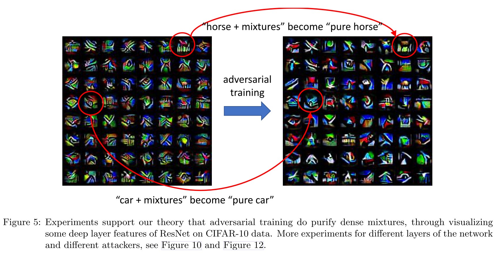
One critical observation is that such dense mixture $v$ has low correlation with almost all inputs $x$ from the original distribution, so it has negligible effect for clean accuracy.

However, such dense mixture is extremely vulnerable to small but dense adversarial perturbations of the input along this direction $v$, making the model non-robust.

As shown in Figure 5:

As we point out, such “dense adversarial perturbation” directions do not exist in the original data. Thus, one has to rely on adversarial training to remove dense mixtures to make the model robust.

They also state the source of dense mixture:

At a high level, in each iteration, the gradient $\nabla\bold{Obj}$ will bias towards the direction that correlates with the labeling function $y=\text{sign}(\left<w^*,z\right>)$; and since $x=\bold{M}z+\xi$ in our model, such directions should be $\bold{M}w^*=\sum_{j}w_j^*\bold{M}_j$, so it a dense mixture direction and will be accumulated across time.

It seems to indicate that labeling function misguides the learning algorithm to learn the dense mixture.

Adversarial Training

Theorem 5.3 (adversarial training, sketched). In the same setting as Theorem 5.1, suppose $A$ is an $\ell_2$ perturbation algorithm with radius $\tau\le\frac{1}{k^{0.5+c}}$. Suppose we run clean training Algorithm 1 for $T_f\ge T_c$ iterations followed with adversarial training Algorithm 2 for $T_g=\Theta(\frac{k^{2+c}}{\eta})$ iterations.

The following holds with high probability:

1. Empirical robust accuracy: for $t=T_f+T_g$

   $$\hat{\varepsilon_t^r}=\bold{Pr}_{x,y=y(x),\rho,r}[\text{sign}(f_t(x+A(f_t,x,y,r)))\neq y]\le o(1)$$

2. Provable robust accuracy: when $A$ is the fast gradient method (FGM), for $t=T_f+T_g$

   $$\varepsilon_t^r:=\bold{Pr}_{x,y=y(x),\rho}[\exist\delta\in\R^d,||\delta||_2\le\tau:\text{sign}(f_t(x+\delta))\neq y]\le o(1)$$

3. Feature (local) purification: for every $t\in[T_f,T_f+T_g-1]$,

   $$\sum_{i\in[m]}||w_i^{(T_f)}-w_i^{(t)}||_2^2=o(1)\times\sum_{i\in[m]}||w_i^{(T_f)}||_2^2$$

   ???

More surprisingly, Theorem 5.3b says when a good perturbation algorithm such as FGM is used, then not only the robustness generalizes to unseen examples, it also generalizes to any worst-case perturbation algorithm.

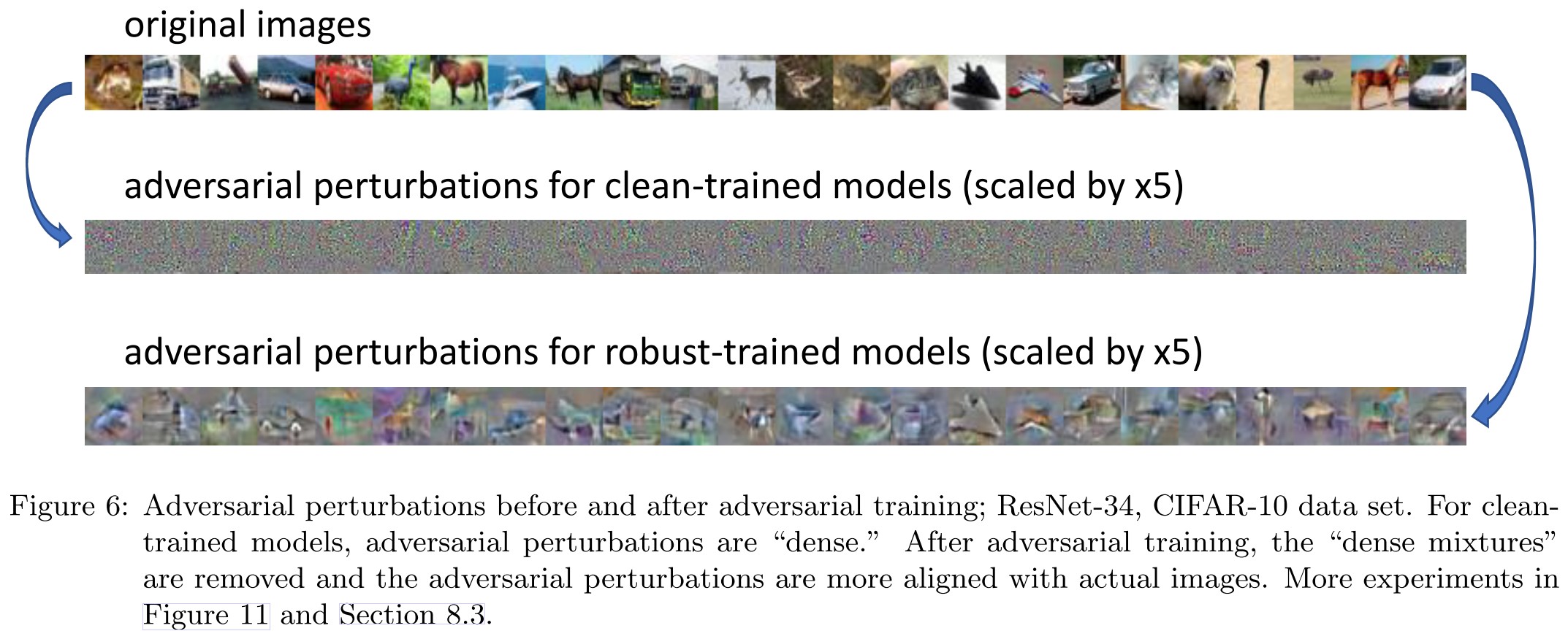
As shown in Figure 6:

Our theorem shows one of the main goals of adversarial training is to remove dense mixtures to make the network more robust. Therefore, before adversarial training, the adversarial perturbations are dense in the basis of $\{\bold{M}_j\}_{j\in[d]}$; and after adversarial training, the adversarial perturbations ought to be more sparse and aligned with inputs from the original data set.

It says that adversarial training does not eliminate the adversarial perturbations, instead, it spreads the adversarial perturbations, making the perturbations semantically meaningful, violating the imperceptibility.

L_∞ Robustness and Lower Bound for Low-Complexity Models

Theorem 5.4 ($\ell_{\infty}$ adversarial training, sketched). Suppose $||\bold{M}||_{\infty},||\bold{M}||_1=d^{o(1)}$. There exists constant $c_1\in(0,c_0)$, such that, in the same setting as Theorem 5.3, except now for any $k\in[d^{c_1},d^{0.399}]$, and $A$ is an $\ell_{\infty}$-perturbation algorithm with radius $\tau=\frac{1}{k^{1.75+2c_0}}$. Then, the same Theorem 5.3 and Theorem 5.1 still hold and imply:

• clean training is not robust against $\ell_{\infty}$-perturbation with radius $\frac{1}{k^{2-c_1}}$.
• adversarial training is robust against any $\ell_{\infty}$-perturbation of radius $\frac{1}{k^{1.75+2c_0}}$

This gives a gap because $c_0,c_1$ can be made arbitrarily small.

???

Definition 5.5 The feature mapping of the neural tangent kernel for out two-layer network $f$ is

Therefore, given weights $\{v_i\}_{i\in[m]}$, the NTK (neural tangent kernel) function $p(x)$ is given as

Without loss of generality, assume each $w_i\sim\mathcal{N}(0,\bold{I})$.

???

They prove the following:

Theorem 5.6 (lower bound). For every constant $C>1$, suppose $m\le d^C$, then there is a constant $c>0$ such that when $k=\frac{1}{d^c}$, considering $\ell_{\infty}$-perturbation with radius $\tau=\frac{1}{k^{100}}$, we have w.h.p. over the choice of $w_i$, for every $p(x)$ in the above definition, the robust error

And the following corollary:

Corollary 5.7 (lower bound). In the same setting as Theorem 5.6, if $q(x)$ is a constant degree polynomial, then we have the robust error $\varepsilon^r(q)\ge\frac{1-o(1)}{2}$.

I cannot get any sense.....

Overview of the Training Process

Lottery ticket winning

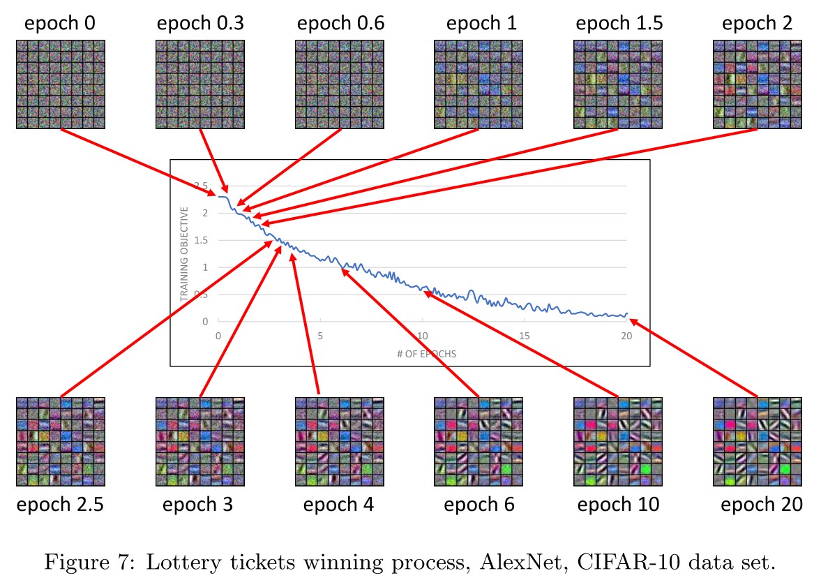
In other words, even with very mild over-parameterization $m\ge d^{1.01}$,by the property of random Gaussian initialization, there will be some “potentially lucky neurons” in (ii), where the maximum correlation to one of the features $\bold{M}_j$ is slightly higher than usual

Lottery tickets winning process For every $j\in[d]$, at every iteration $t$, if $i\in\mathcal{S}_{j,sure}^{(0)}$, then $\left<\bold{M}_j,w_i^{(t)}\right>^2$ will grow faster than $\left<\bold{M}_j^\prime,w_i^{(t)}\right>^2$ for every $t$, until $\left<\bold{M}_j,w_i^{(t)}\right>^2$ becomes sufficiently larger than all the other $\left<\bold{M}_j^\prime,w_i^{(t)}\right>^2$.

In other words, if neuron $i$ wins the lottery ticket at random initialization, then eventually, it will deviate from random initialization and grow to a feature that is more close to (a scaling of) $\bold{M}_j$.

Some neurons will be lucky to resemble the feature mostly at begining and grows into the feature responsible neuron.

Dense mixture

We shall prove that in this phase, gradient descent will also accumulate, in each neuron, a small “dense mixture” that is extremely vulnerable to small but adversarial perturbations.

If a neuron i wins the lottery ticket for feature $\bold{M}_j$ near random initialization, then it will keep this “lottery ticket” throughout the training.

But they show that that even for the “lucky neuron” that wins the lottery ticket, the hidden weight of this neuron will look like:

i.e. the weight will be like $w_i\approx \bold{M}_j+v_i$, where $v_i$ is a "dense mixture":

Their key observation is that $v_i$ is small and dense, i.e. with high probability:

This dense mixture will not be correlated with any particular natural input, and thus the existence of these mixtures will have negligible contribution to the output of ft on clean data.

But it's possible to create a correlated perturbation along the dense direction $\delta\propto \sum_{j^\prime\in[d]}\bold{M}_{j^\prime}$, i.e.

Thus, at this phase, even when the network has a good clean accuracy, it is still non-robust to these small yet dense adversarial perturbations.

Moreover, this perturbation direction is “universal”, in the sense that it does not depend on the randomness of the model at initialization, or the randomness we use during the training. This explains transfer attacks in practice: that is, the adversarial perturbation found in one model can also attack other models that are independently trained.

Since Eq. (6.2) suggests most original inputs have negligible correlations with each dense mixture, during clean training, gradient descent will have no incentive to remove those mixtures.

They point out that it's a property of gradient descent:

We emphasize that this is indeed a special property of gradient descent.

(Stochastic) gradient descent, as a local update algorithm, only exams the local correlation between the update direction and the labeling function, and it does not exam whether this direction can be used in the final result.

In fact, even if we use $w_i=\bold{M}_i$ as initialization as opposed to random initialization, continuing clean training will still accumulate these small but dense mixtures.

Local learning accumulates noise?

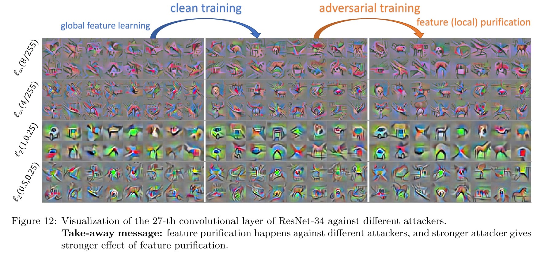
More experiments results

Inspirations

They propose a principle named as feature purification to describe what adversarial training is doing to the cleanly trained models.

They point out that gradient descent will accumulate dense mixtures correlated to the labeling function into the features learned, which is less correlated with inputs, therefore hurting no accuracy, but correlated perturbations towards the direction of dense mixtures lead to mistakes, making the model adversarially vulnerable.

Adversarial training instead is able to remove these dense mixtures, thus purifying the features learned by model.

It seems that adversarial training indeed does not eliminate adversarial examples, but amplify the perturbations required and spread the perturbations in a semantically meaningful way.

It also seems to indicate that a better labeling function can improve adversarial robustness.