First-order Adversarial Vulnerability

By LI Haoyang 2020.11.16

Content

First-order Adversarial Vulnerability - ICML 2019

Code:https://github.com/facebookresearch/AdversarialAndDimensionality

Carl-Johann Simon-Gabriel, Yann Ollivier, Léon Bottou, Bernhard Schölkopf, David Lopez-Paz. First-order Adversarial Vulnerability of Neural Networks and Input Dimension. ICML 2019. arXiv:1802.01421

We show that adversarial vulnerability increases with the gradients of the training objective when viewed as a function of the inputs.

Surprisingly, vulnerability does not depend on network topology.

We empirically show that this dimension dependence persists after either usual or robust training, but gets attenuated with higher regularization.

Their contributions:

• We show an empirical one-to-one relationship between average gradient norms and adversarial vulnerability.
• We formally prove that, at initialization, the first-order vulnerability of common neural networks increases as $\sqrt{d}$ with input dimension $d$.
• We empirically show that this dimension dependence persists after both usual and robust (PGD) training, but gets dampened and eventually vanishes with higher regularization.
• We observe that further training after the training loss has reached its minimum can provide improved test accuracy, but severely damages the network’s robustness.
• We notice a striking discrepancy between the gradient norms (and therefore the vulnerability) on the training and test sets respectively.

From Adversarial Examples to Large Gradients

Adversarial example is a small perturbation of the inputs that creates a large variation of outputs.

Given a classifier $\varphi$ and an input image $x$, an adversarial image is constructed by adding a perturbation $\delta$ such that $||\delta||\le \epsilon$ and $\varphi(x+\delta)\neq \varphi(x)$.

Definition 1 Given a distribution $P$ over the input-space, we call adversarial vulnerability of a classifier $\varphi$ to an $\epsilon$-sized $||\cdot||$-attack the probability that there exists a perturbation $\delta$ of $x$ such that

The adversarial ($\mathcal{L-}$) damage is defined as the average increase-after-attack, i.e. $\Bbb{E}_{x\sim P}[\Delta\mathcal{L}]$ of a loss $\mathcal{L}$. When $\mathcal{L}$ is the 0-1 loss $\mathcal{L}_{0/1}$, adversarial damage is the accuracy-drop after attack, which lower bounds adversarial vulnerability.

The accuracy-drop rules out natural adversarial examples, thus lower bounds the adversarial vulnerability.

In practice, a smoother surrogate loss $\mathcal{L}$ is used instead of the non-differentiable 0-1 loss. Hence, a classifier $\varphi$ will be robust if, on average over $x$, a small adversarial perturbation $\delta$ of $x$ creates only a small variation $\delta\mathcal{L}$ of the loss. (It can also be the case of obfuscated gradient.)

If $||\delta||\le \epsilon$, then a first order Taylor expansion in $\epsilon$ shows that

where $\partial_{x}\mathcal{L}$ denotes the gradient of $\mathcal{L}$ with respect to $x$ and $|||\cdot|||$ denotes the dual norm of $||\cdot||$.

The dual norm is defined as:

which obviously explains the last equality.

The dual norm of $||\cdot||_1$ is $||\cdot||_{\infty}$, and the dual norm of $||\cdot||_p$ is $||\cdot||_q$, such that $\frac{1}{p}+\frac{1}{q}=1$.

This leads to the following lemma.

Lemma 2 At first order approximation in $\epsilon$, an $\epsilon$-sized adversarial attack generated with norm $||\cdot||$ increase the loss $\mathcal{L}$ at point $x$ by $\epsilon|||\partial_{x}\mathcal{L}|||$, where $|||\cdot|||$ is the dual norm of $||\cdot||$. In particular, an $\epsilon$-sized $\ell_p$-attack increases the loss by $\epsilon||\partial_{x}\mathcal{L}||_q$, where $1\le q\le\infty$ and $\frac{1}{p}+\frac{1}{q}=1$.

Moreover, we will see that the first-order predictions closely match the experiments.

This lemma shows that adversarial vulnerability depends on three main factors:

• $||\cdot||$, the chosen norm of threat model

  A measure of sensibility to image perturbations.

• $\epsilon$, the size of attack

  A sensibility threshold.

• $\Bbb{E}_{x}|||\partial_{x}\mathcal{L}|||$, the expected dual norm of $\partial_x\mathcal{L}$

  The classifier's expected marginal sensibility to a unit perturbation.

For a given pixel-wise order of magnitude of the perturbations $\delta$, the $\ell_p$-norm of the perturbation will scale like $d^{1/p}$, which suggests that the threshold $\epsilon_p$ used with $\ell_p$-attacks can be written as

in which, $\epsilon_{\infty}$ denotes a dimension independent constant.

This scaling also preserves the average signal-to-noise ratio $||x||_2/||\delta||_2$.

A new old regularizer (defenses inspired by Lemma 2)

Lemma 2 shows that the loss of the network after an $\frac{\epsilon}{2}$-sized $||\cdot||$-attack is

It is thus natural to take this loss-after-attack as a new training objective.

In the case that $||\cdot||=||\cdot||_2$, this new loss reduces to an old regularization scheme proposed by Drucker & LeCun (1991) called double backpropagation.

A priori, we do not know what will happen for attacks generated with other norms; but our experiments suggest that training with one norm also protects against other attacks.

Link to adversarially augmented training

When augmenting the training set with online generated $\epsilon$-sized $||\cdot||$-attacks $x+\delta$, the training objectively is

referred as adversarially augmented training by the authors. (Generally known as adversarial training.)

They prove that this 'old-plus-post-attack' loss simply reduces to the loss-after-attack loss using the first order Taylor expansion.

Proposition 3 Up to first-order approximations in $\epsilon$, $\tilde{\mathcal{L}}_{\epsilon,||\cdot||}=\mathcal{L}_{\epsilon,|||\cdot|||}$. Said differently, for small enough $\epsilon$, adversarially augmented training with $\epsilon$-sized $||\cdot||$-attacks amounts to penalizing the dual norm $|||\cdot|||$ of $\partial_{x}\mathcal{L}$ with weight $\epsilon/2$. In particular, double-backpropagation corresponds to training with $\ell_2$-attacks, while FGSM-augmented training corresponds to an $\ell_1$-penalty on $\partial_{x}\mathcal{L}$.

This correspondence between training with perturbations and using a regularizer can be compared to Tikhonov regularization: Tikhonov regularization amounts to training with random noise Bishop (1995), while training with adversarial noise amounts to penalizing $\partial_{x}\mathcal{L}$.

Evaluate Adversarial Vulnerability

One Neuron with Many Inputs

Suppose for a moment that the coordinates of $\partial_{x}\mathcal{L}$ have typical magnitude $|\partial_x\mathcal{L}|$, then $||\partial_x\mathcal{L}||_q$ scales like $d^{1/q}|\partial_x\mathcal{L}|$, consequently

The second and the last are bridged by $\epsilon_p\propto d^{1/p}$ and $\frac{1}{q}+\frac{1}{p}=1$.

It shows that to be robust against any type of $\ell_p$-attack at any input-dimension $d$, the average absolute value of the coefficients of $\partial_x\mathcal{L}$ must grow slower than $1/d$. (Is it true?)

The neural weights are usually initialized with a variance that is inversely proportional to the number of inputs per neuron.

Consider the case when one output neuron $o$ is connected to all input pixels, given the initialization with a variance of $1/d$, the average absolute value $|\partial_x o|\equiv|\partial_x\mathcal{L}|$ grows like $1/\sqrt{d}$, thus the adversarial vulnerability $\epsilon||\partial_x o||_q\equiv\epsilon||\partial_x\mathcal{L}||_q$ increases like $d/\sqrt{d}=\sqrt{d}$.

Intuitively, the above sounds reasonable, but a more detailed illustration is needed to be more convincing.

This toy example shows that the standard initialization scheme, which preserves the variance from layer to layer, causes the average coordinate-size $|\partial_x\mathcal{L}|$ to grow like $1/\sqrt{d}$ instead of $1/d$. When an $\ell_{\infty}$-attack tweaks its $\epsilon$-sized input perturbations to align with the coordinate-signs of $\partial_x\mathcal{L}$, all coordinates of $\partial_x\mathcal{L}$ add up in absolute value, resulting in an output-perturbation that scales like $\epsilon\sqrt{d}$ and leaves the network increasingly vulnerable with growing input-dimension.

Formal Statements for Deep Networks

These statements are based on the following set $\mathcal{H}$ of hypotheses:

• H1 Non-input neurons are followed by a ReLU killing half of its inputs, independently of the weights.
• H2 Neurons are partitioned into layers, meaning groups that each path traverses at most once.
• H3 All weights have 0 expectation and variance 2/(in-degree) (‘He-initialization’).
• H4 The weights from different layers are independent.
• H5 Two distinct weights $w,w^\prime$ from a same node satisfy $\Bbb{E}[w w^\prime]=0$.

Not covering all cases, but reasonable.

Nevertheless, they do not hold after training. That is why all our statements in this section are to be understood as orders of magnitudes that are very well satisfied at initialization both in theory and practice.

Theorem 4 (Vulnerability of Fully Connected Nets) Consider a succession of fully connected layers with ReLU activations which takes inputs $x$ of dimension $d$, satisfies assumptions $\mathcal{H}$, and outputs logits $f_k(x)$ that get fed to a final cross-entropy-loss layer $\mathcal{L}$. Then the coordinated of $\partial_x f_k$ grow like $1/\sqrt{d}$, and

These networks are thus increasingly vulnerable to $\ell_p$-attacks with growing input-dimension.

For a given path $p$, let the path-degree $d_p$ be the multiset of encountered in-degrees along path $p$. For a fully connected network, this is the unordered sequence of layer-sizes preceding the last path-node, including the input-layer.

Choose a path of calculation, put each node's in-degrees into a set.

Consider the multiset $\{d_p\}_{p\in\mathcal{P}(x,o)}$ of all path-degrees when $p$ varies among all paths from input $x$ to output $o$. The symmetry assumption is

($\mathcal{S}$) All input nodes $x$ have the same multiset $\{d_p\}_{p\in\mathcal{P}(x,o)}$ of path-degrees from $x$ to $o$.

Intuitively, this means that the statistics of degrees encountered along paths to the output are the same for all input nodes. This symmetry assumption is exactly satisfied by fully connected nets, almost satisfied by CNNs (up to boundary effects, which can be alleviated via periodic or mirror padding) and exactly satisfied by strided layers, if the layersize is a multiple of the stride.

Theorem 5 (Vulnerability of Feedforward Nets). Consider any feedforward network with linear connections and ReLU activation functions. Assume the net satisfies assumptions $\mathcal{H}$ and output logits $f_k(x)$ that get fed to the cross-entropy-loss $\mathcal{L}$. Then $||\partial_x f_k||_2$ is independent of the input dimension $d$ and $\epsilon_2||\partial_x\mathcal{L}||_2\propto \sqrt{d}$. Moreover, if the net satisfies the symmetry assumption $\mathcal{S}$, then $|\partial_x f_k|\propto 1/\sqrt{d}$ , $||\partial_x\mathcal{L}||_q\propto d^{\frac{1}{q}-\frac{1}{2}}$ and $\epsilon_p||\partial_x\mathcal{L}||_q\propto\sqrt{d}$.

The main proof idea is that in the gradient norm computation, the He initialization exactly compensates the combinatorics of the number of paths in the network, so that this norm becomes independent of the network topology.

Corollary 6 (Vulnerability of CNNs) In any succession of convolution and dense layers, strided or not, with ReLU activations, that satisfies assumptions $\mathcal{H}$ and outputs logits that get fed to the cross-entropy-loss $\mathcal{L}$, the gradient of the logit-coordinates scale like $1/\sqrt{d}$ and (7) (results in theorem 4) is satisfied. It is hence increasingly vulnerable with growing input-resolution to attacks generated with any $\ell_p$-norm.

Although the principles of our analysis naturally extend to residual nets, they are not yet covered by our theorems.

Current weight initializations (He-, Glorot-, Xavier-) are chosen to preserve the variance from layer to layer, which constrains their scaling to 1/√ in-degree.

Also note that rescaling all weights by a constant does not change the classification decisions, but it affects cross-entropy and therefore adversarial damage.

Empirical Results

First-Order Approximation, Gradient Penalty, Adversarial Augmentation

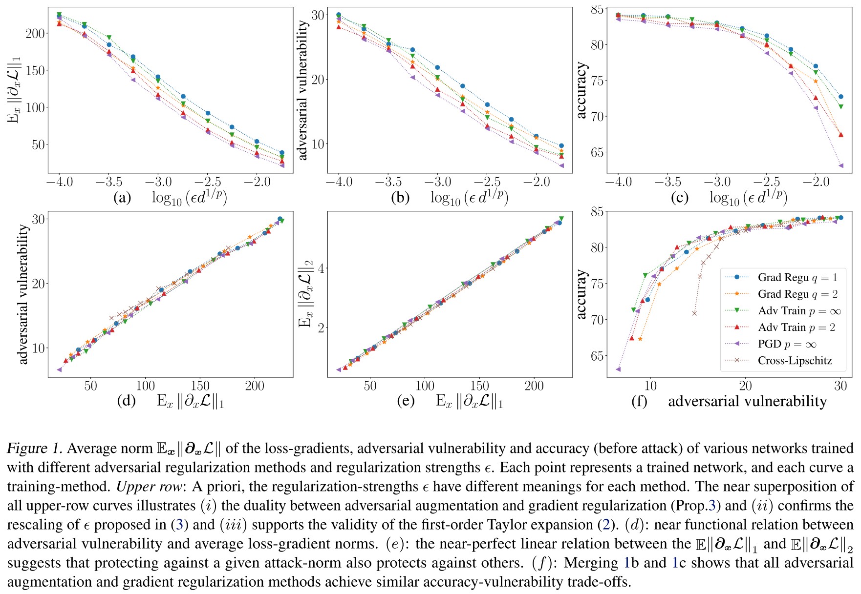
We train several CNNs with same architecture to classify CIFAR-10 images (Krizhevsky, 2009). For each net, we use a specific training method with a specific regularization value $\epsilon$.

Note that our goal here is not to advocate one defense over another, but rather to check the validity of the Taylor expansion, and empirically verify that first order terms (i.e., gradients) suffice to explain much of the observed adversarial vulnerability.

As shown in Figure 1, they have following conclusions:

1. Confirming first order expansion and large first-order vulnerability

   • the efficiency of the first-order defense against iterative (non-first-order) attacks (Fig.1&4a).
   • the striking similarity between the PGD curves (adversarial augmentation with iterative attacks) and the other adversarial training training curves (one-step attacks/defenses).
   • the functional-like dependence between any approximation of adversarial vulnerability and $\Bbb{E}_x||\partial_x\mathcal{L}||_1$ (Fig.4b), and its independence on the training method
   • the excellent correspondence between the gradient regularization and adversarial augmentation curves (see next paragraph).

2. Gradient regularization matches adversarial augmentation

3. Confirming correspondence of norm-dependent thresholds

4. Accuracy-vulnerability trade-off: confirming large first-order component of vulnerability

5. The regularization-norm does not matter

Vulnerability’s Dependence on Input Dimension

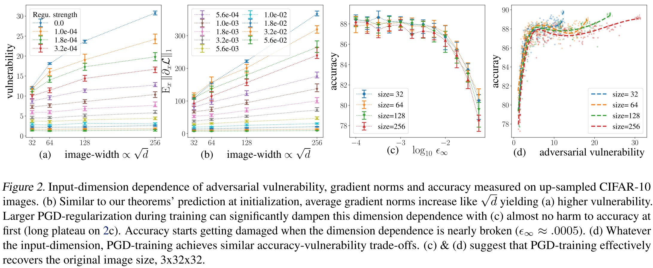
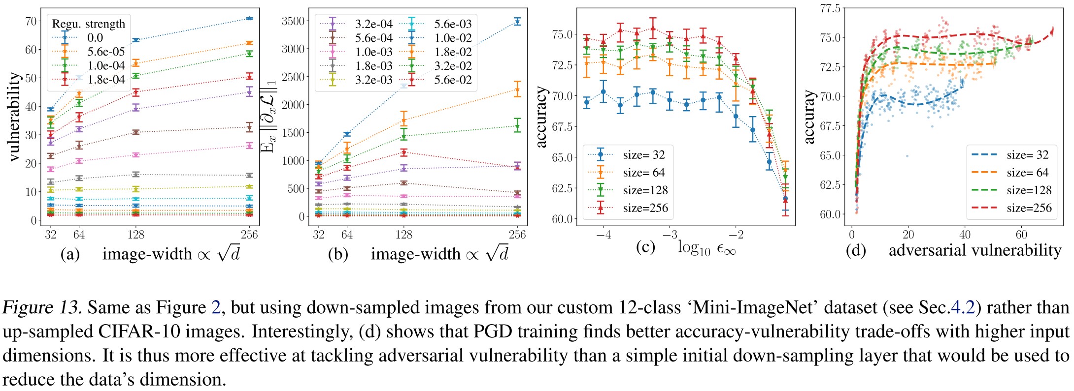
Theorems 4-5 and Corollary 6 predict a linear growth of the average $\ell_1$-norm of $\partial_x\mathcal{L}$ with the square root of the input dimension $d$, and therefore an increased adversarial vulnerability (Lemma 2).

As shown in Figure 2 and Figure 13, they have the following conclusions:

1. Gradients and vulnerability increase with $\sqrt{d}$. ( Figure 2 (a) and (b))

2. Accuracies are dimension independent ( Figure 2 (c))

   This hints to defend using dimension manipulation.

3. PGD effectively recovers original input dimension ( Figure 2 (d))

   Higher dimensions have a longer plateau to the right, because without regularization, vulnerability increases with input dimension.

   The curves overlap when moving to the left, meaning that the accuracy vulnerability trade-offs achieved by PGD are essentially independent ofthe actual input dimension.

4. PGD training outperforms down-sampling (Figure 13.)

Further Experiments

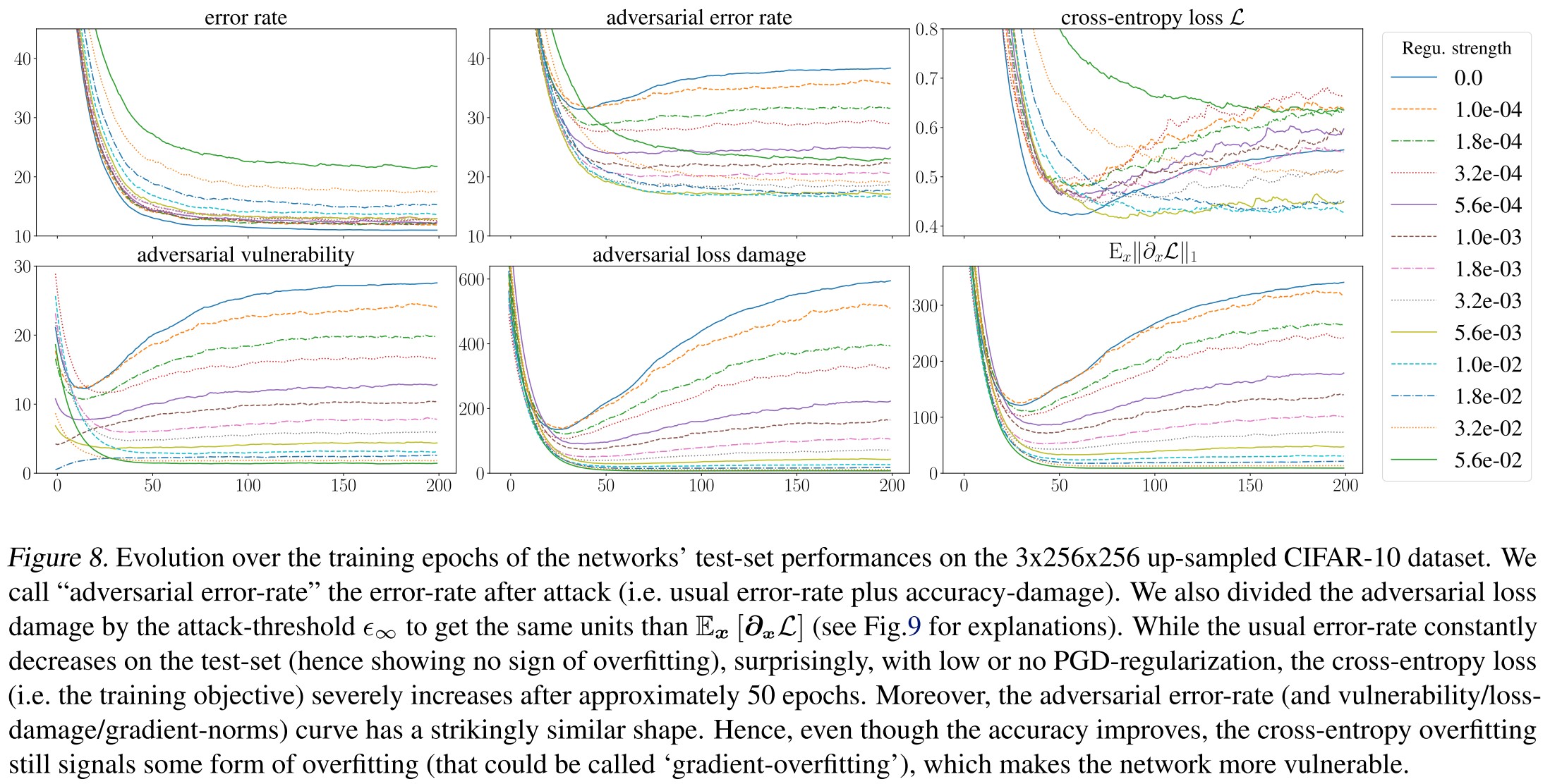
As shown in Figure 8, they have the following conclusions:

1. Non-equivalence of loss- and accuracy-damage. (Figure 8 a & c)

   The test-error continues to decrease all over training, while the cross-entropy increases on the test set from epoch ≈ 40 and on.

   Intriguing.

2. Early stopping dampens vulnerability

   Since cross-entropy overfits, early stopping effectively acts as a defense. (Figure 10)

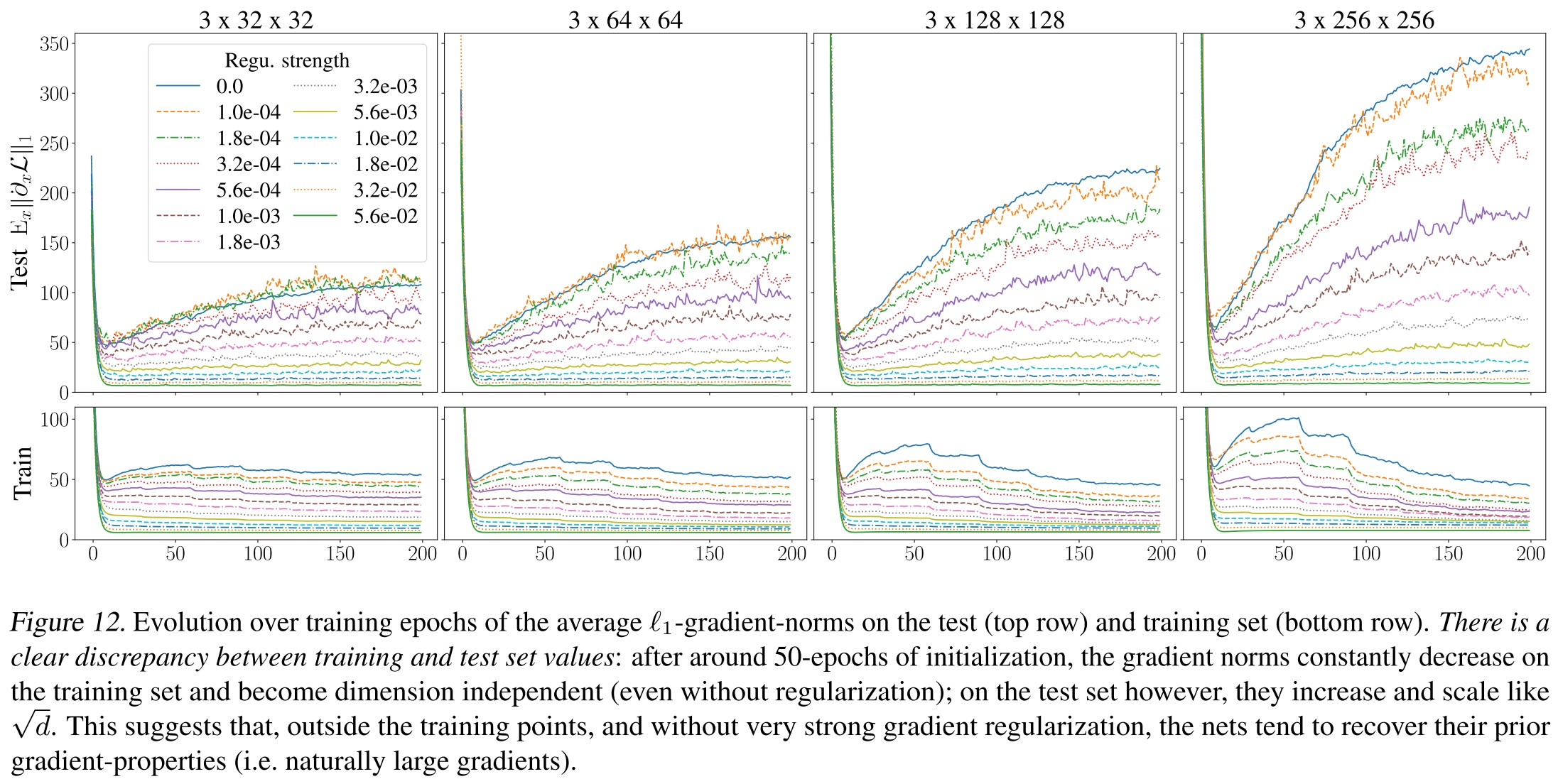
As shown in Figure 12,

Gradient norms do not generalize well

This discrepancy increases over training (gradient norms decrease on the training data but increase on the test set).

Inspirations

This paper is very informative. It bridges up the regularization with adversarial training and give many fruitful insights.

I think the subsequent defenses can cut in from the following perspectives:

• The dimension of inputs
• Regularization of gradients (JARN, GradAlign, etc.)
• New structure
• Improvement of adversarial training (as verified by this paper)