Adversarial Vulnerability

By LI Haoyang 2020.10.27

Adversarial vulnerability for any classifier - NIPS 2018

Paper: http://papers.nips.cc/paper/7394-adversarial-vulnerability-for-any-classifier

Alhussein Fawzi, Hamza Fawzi, Omar Fawzi. Adversarial vulnerability for any classifier. NIPS 2018.

In this paper, we study the phenomenon of adversarial perturbations under the assumption that the data is generated with a smooth generative model. We derive fundamental upper bounds on the robustness to perturbations of any classification function, and prove the existence of adversarial perturbations that transfer well across different classifiers with small risk.

Setting

Generator and classifier

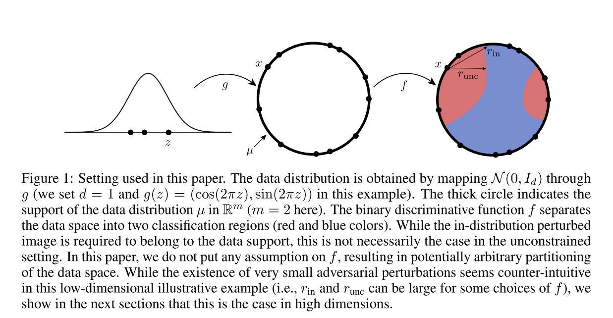
A generative model $g$ maps latent vectors $z\in\cal{Z}:=\R^d$ into the space of images $\cal{X}:=\R^m$ of $m$ pixels, i.e.

To generate an image according to the distribution of natural images $\mu$, a random vector $z\sim \upsilon$ is sampled from a Gaussian distribution $\upsilon=\mathcal{N}(0,I_d)$ and then mapped to the space of image, i.e. $g(z)$.

A classifier $f$ maps images in $\cal{X}:=\R^m$ to discrete labels $\{1,\dots,K\}$, i.e.

The discriminator $f$ partitions $\cal{X}$ into $K$ sets $C_i=\{x\in\cal{X}:f(x)=i\}$, each of which corresponds to a different predicted label.

The relative proportion of points in class $i$ is equal to

i.e. the Gaussian measure of $g^{-1}(C_i)$ in $\cal{Z}$.

The goal of this paper is to study the robustness of $f$ to additive perturbations under the assumption that the data is generated according to $g$.

Robustness

They define two notions of robustness.

• In-distribution robustness

  For $x=g(z)$, the in-distribution robustness $r_{in}(x)$ is defined as

  $$r_{in}(x)=\min_{r\in\mathcal{Z}}||g(z+r)-x||,s.t.f(g(z+r))\ne f(x)$$

  In short, the minimal perturbation added to original image that change the classification result while remain the perturbed image in the original distribution of images.

• Unconstrained robustness

  The unconstrained robustness is the general definition of adversarial perturbations, i.e.

  $$r_{unc}(x)=\min_{r\in\mathcal{X}}||r||,s.t. f(x+r)\ne f(x)$$

  It is easy to see that this robustness definition is smaller than the in-distribution robustness, i.e. $r_{unc}(x)\le r_{in}(x)$. (why?)

They assume that the generative model is smooth in the sense that it satisfies as modulus of continuity property:

Assumption 1 We assume that $g$ admits a monotone invertible modulus of continuity $w$, i.e.

Note that the above assumption is milder than assuming Lipschitz continuity. In fact, the Lipschitz property corresponds to choosing $w(t)$ to be a linear function of $t$. In particular, the above assumption does not require that $w(0)=0$, which potentially allows us to model distributions with disconnected support.

Upper bounds on robustness

Theorem 1. Let $f:\R^m\to\{1,\dots,K\}$ be an arbitrary classification function defined on the image space. Then, the function of datapoints having robustness less than $\eta$ satisfies

where $\Phi$ is the cdf (累积分布函数) of $\cal{N}(0,1)$, i.e. $\Phi(x)=\frac{1}{\sqrt{2\pi}}\int_{-\infty}^xe^{-u^2/2}du$, and $a_{\ne i}=\Phi^{-1}\left(\Bbb{P}\left(\cup_{i\ne i}C_i\right)\right)$.

In particular, if for all $i$, $\Bbb{P}(C_i)\le\frac{1}{2}$ (the classes are not too unbalanced), we have

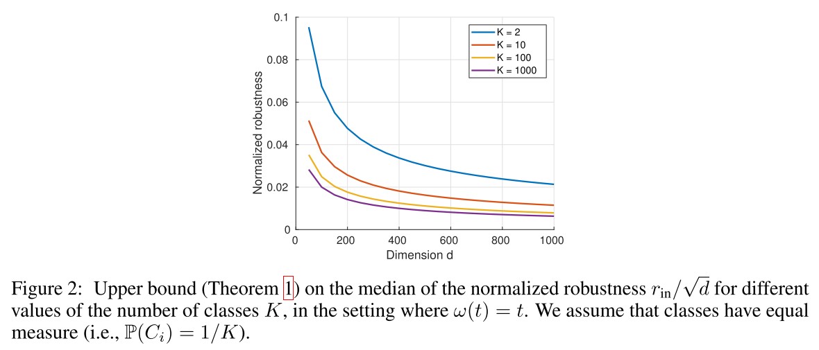
To see the dependence on the number of classes more explicitly, consider the setting where the classes are equiprobable, i.e. $\Bbb{P}(C_i)=\frac{1}{K}$ for all $i, K\ge 5$, then

Based on Theorem 1, there are following results

• Interpretaion with $w^{-1}(\eta)=\eta/L$

  

  Our result shows that when $d$ is large and $g$ is smooth (i.e. $L\ll d$, $L$ is the Lipschitz constant), there exist small adversarial perturbations that can fool arbitrary classifiers $f$.

• Dependence on $K$

  In other words, it is easier to find adversarial perturbations in the setting where the number of classes is large, than for a binary classification task.

• Classification-agnostic bound

  Our bounds hold for any classification function $f$.

• How tight is the upper bound?

  This suggests that classifiers are maximally robust when the induced classification boundaries in the latent space are linear.

Relation between in-distribution robustness and unconstrained robustness

It's possible to construct a family of classifiers for which $r_{unc}(x)\ge\frac{1}{2}r_{in}(x)$.

For a given classifier $f$ in the image space, define the classifier $\tilde{f}$ constructed in a nearest neighbor strategy:

Theorem 2. For the classifier $\tilde{f}$, we have $r_{unc}(x)\ge\frac{1}{2}r_{in}(x)$.

This result shows that if a classifier has in-distribution robustness $r$, then we can construct a classifier with unconstrained robustness $\frac{r}{2}$, through a simple modification of the original classifier $f$.

This suggests that the unconstrained robustness can be increased by increasing in-distribution robustness.

Transferability of perturbations

Theorem 3 (Transferability of perturbations). Let $f,h$ be two classifiers. Assume that $\Bbb{P}(f\circ g(z)\neq h\circ g(z))\le\delta$ (e.g. if $f$ and $h$ have a risk bounded by $\delta/2$ for the data set generated by $g$). In addition, assume that $\Bbb{P}(C_i(f))+\delta\le \frac{1}{2}$ for all $i$, then

Compared to Theorem 1 which bounds the robustness to adversarial perturbations, the extra price to pay here to find transferable adversarial perturbations is the $2\delta$ term, which is small if the risk of both classifiers is small.

This suggests that if both classifiers are easy to be fooled, it's not that difficult to find a transferable adversarial example.

Approximate generative model

Theorem 4. We use the same notations as in Theorem 1. Assume that the generator $g$ provides a $\delta$ approximation of the true distribution $\mu$ in the $1$-Wasserstein sense on the metric space $(\cal{X},||\cdot||)$; that is, $W(g_{*}(\upsilon),\mu)\le\delta$ (where $g_{*}(\upsilon)$ is the pushforward of $\upsilon$ via $g$), the following inequality holds provided $w$ is concave

where $r_{unc}(x)$ is the unconstrained robustness in the image space. In particular, for $K\ge 5$ equiprobable classes, we have

In words, when the data is defined according to a distribution which can be approximated by a smooth, high-dimensional generative model, our results show that arbitrary classifiers will have small adversarial examples in expectation.

We also note that as $K$ grows, this bound decreases and even goes to zero under the sole condition that $w$ is continuous at $0$. Note however that the decrease is slow as it is only logarithmic.

This suggests that for a classification of infinity classes, the expected adversarial perturbation can be very small.

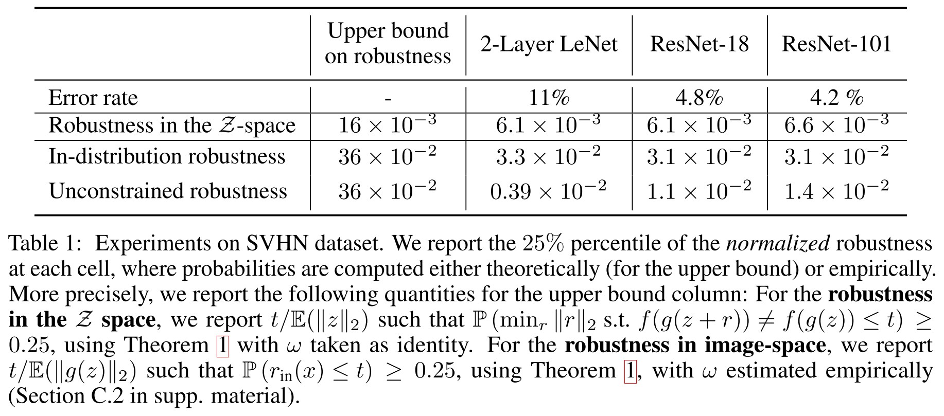
Experiments

Inspirations

I admit that I don't completely understand this paper.

From the general idea, this paper suggests the following potentials

• Higher-dimensional data and more classes introduce less robustness.
• Unconstrained robustness (general robustness) can be increased by increasing in-distribution robustness (It seems to suggest that an accurate model is also important in terms of robustness?)
• A classifier is more robust if the boundary in latent space is more linear.

Derivation of theorems

Gaussian isoperimetric inequality

The standard Gaussian distribution is

Theorem

Let $\upsilon_d$ be the Gaussian measure on $\R^d$. Let $A\sube \R^d$ and let $A_{\eta}=\{z\in\R^d:\exist z^{'}\in A,s.t. ||z-z^{'}||_2\le\eta\}$. If $\upsilon_d(A)=\Phi(a)$, then $\upsilon_d(A_{\eta})\ge\Phi(a+\eta)$.

In words, $A_{\eta}$ is a subset of points in $A$ such that every point in $A_{\eta}$ has at least a neighbor in $A$ closer than $\eta$ in terms of $||\cdot||_2$, the theorem says that if the probability that $A$ is sampled is $\Phi(a)$, the probability that $A_{\eta}$ is sampled is higher than $\Phi(a+\eta)$.

Theorem 1

Theorem

Let $f:\R^m\to\{1,\dots,K\}$ be an arbitrary classification function defined on the image space. Then, the function of datapoints having robustness less than $\eta$ satisfies

where $\Phi$ is the cdf (累积分布函数) of $\cal{N}(0,1)$, i.e. $\Phi(x)=\frac{1}{\sqrt{2\pi}}\int_{-\infty}^xe^{-x^2/2}dx$, and $a_{\ne i}=\Phi^{-1}\left(\Bbb{P}\left(\cup_{i\ne i}C_i\right)\right)$.

In particular, if for all $i$, $\Bbb{P}(C_i)\le\frac{1}{2}$ (the classes are not too unbalanced), we have

To see the dependence on the number of classes more explicitly, consider the setting where the classes are equiprobable, i.e. $\Bbb{P}(C_i)=\frac{1}{K}$ for all $i, K\ge 5$, then

Derivation

First, define

In short, $dist(x,C)$ is the distance between $x$ and the closest data in $C$, therefore, $C_{i\to}$ is a set of data points classified as $C_i$ such that their closest distances with data points in other classes are less than $\eta$, it's a set of out-most data points.

Then, define the following sets in the $z$-space

Remind that $w^{-1}(\eta)$ maps the upper bound $\eta$ into the $z$-space.

It's easy to verify that $g(B_{i\to})\sube C_{i\to}$.

Thus, we have

Since $C_{i\to}$ is a superset of $B_{i\to}$, the probability of the former is larger than the latter.

Remind the definition of $r_{in}(x)$:

We have

Remind again, $C_{i\to}$ is the set of points that fall into the out-most $\eta$ band, and $r_{in}(x)$ is the minmal distance to move a point from the region corresponding to any class to another region classified some classes else, hence the equation above.

Note that $(B_{i\to})\cup{(\cup_{j\neq i}B_j)}$ is the set of points that are at distance at most $w^{-1}(\eta)$ from $\cup_{j\neq i}B_j$. (by definition)

By the Gaussian isoperimetric inequality applied with $A=\cup_{j\neq i}B_j$ and $a=a_{\neq i}$, ($\upsilon(A)=\Phi(a)$)we have

As $B_{i\to}$ are disjoint for different $i$, we have

And, since $\Bbb{P}(C_{i\to})\ge \upsilon(B_{i\to})$ and $\Bbb{P}(r_{in}(x)\le\eta)=\Bbb{P}(\cup_i C_{i\to})$, there stands the first equation in theorem 1

Intuitively, it says the probability that there exists a data point in $z$-space whose distance to the boundary is closer than $\eta$ is larger than a total probability gain along $w^{-1}(\eta)$.

Theorem 2

Theorem

For a given classifier $f$ in the image space, define the classifier $\tilde{f}$ constructed in a nearest neighbor strategy:

For the classifier $\tilde{f}$, we have $r_{unc}(x)\ge\frac{1}{2}r_{in}(x)$.

The classifier $\tilde{f}$ classifies $x$ as the class of its nearest neighbor in distribution.

Proof

Let $x=g(z)\in\cal{X}$ and $x^{'}\in\cal{X}$. Let $z^*$ be such that $\tilde{f}(x^{'})=f(g(z^*))$. By definition of $\tilde{f}$, we have $||x^{'}-g(z^*)||\le||x^{'}-g(z)||$. As such, using the triangle inequality, we get

Taking the minimum over all $x^{'}$ such that $\tilde{f}(x)\neq\tilde{f}(x^{'})$, we obtain