Are Adversarial Example Inevitable ?

By LI Haoyang 2020.12.8

Content

Are Adversarial Example Inevitable? - ICLR 2019

Ali Shafahi, W. Ronny Huang, Christoph Studer, Soheil Feizi, Tom Goldstein. Are adversarial examples inevitable? ICLR 2019. arXiv:1809.02104

This paper analyzes adversarial examples from a theoretical perspective, and identifies fundamental bounds on the susceptibility of a classifier to adversarial attacks. We show that, for certain classes of problems, adversarial examples are inescapable.

If the image classes each occupy a fraction of the cube greater than $\frac{1}{2}\text{exp}(-\pi \epsilon^2)$, then images exist that are susceptible to adversarial perturbations of $\ell_2$-norm at most.

We present an example image class for which there is no fundamental link between dimensionality and robustness, and argue that the data distribution, and not dimensionality, is the primary cause of adversarial susceptibility.

Notation

The notations they use are as follows:

• $[0,1]^n$, the unit hypercube in $n$ dimensions

• $\text{vol}(\mathcal{A})$, the volume (n-dimensional Lebesgue measure) of a subset $\mathcal{A}\sub [0,1]^n$.

• $\Bbb{S}^{n-1}=\{x\in\R^n|||x||_2 = 1\}$, the unit sphere embedded in $\R^n$.

• $s_{n-1}$, the surface area of $\Bbb{S}^{n-1}$

• $\mu [\mathcal{A}]$, the size of subset $\mathcal{A}\in\Bbb{S}^{n-1}$, i.e. the surface area the set covers

• $\mu_1[\mathcal{A}]=\mu[\mathcal{A}]/s_{n-1}$, the normalized measure, it can be interpreted as the probability of a uniform random point from the sphere lying in $\mathcal{A}$.

• $\ell_p$-norm, i.e.

  $$||z||_p=\left(\sum_i |z_i|^p\right)^{1/p}\text{ if }p>0,\text{ and }||z||_0=\text{card}\{z_i|z_i\neq 0\}$$

Problem Setup

Given data points that lie in a space $\Omega$, the classification problem refers to classify them into $m$ different object classes. These classes are defined by probability density functions $\{\rho_c\}_{c=1}^m$, where $\rho_c:\Omega\to\R$.

A "random" point from class $c$ is a random variable with density $\rho_c$, which is assumed to be upper bounded by $U_c=\sup_x \rho_c(x)$.

A "classifier" function $\mathcal{C}:\Omega\to\{1,2,\dots,m\}$ partitions $\Omega$ into disjoint measurable subsets, one for each class label.

Definition 1 Consider a point $x\in\Omega$ drawn from class $c$, a scalar $\epsilon >0$, and a metric $d$. We say that $x$ admits an $\epsilon$-adversarial example in the metric $d$ if there exists a point $\hat{x}\in\Omega$ with $\mathcal{C}(\hat{x})\neq c$, and $d(x,\hat{x})\le\epsilon$.

The neighborhood of $x$ expands across the classification boundary.

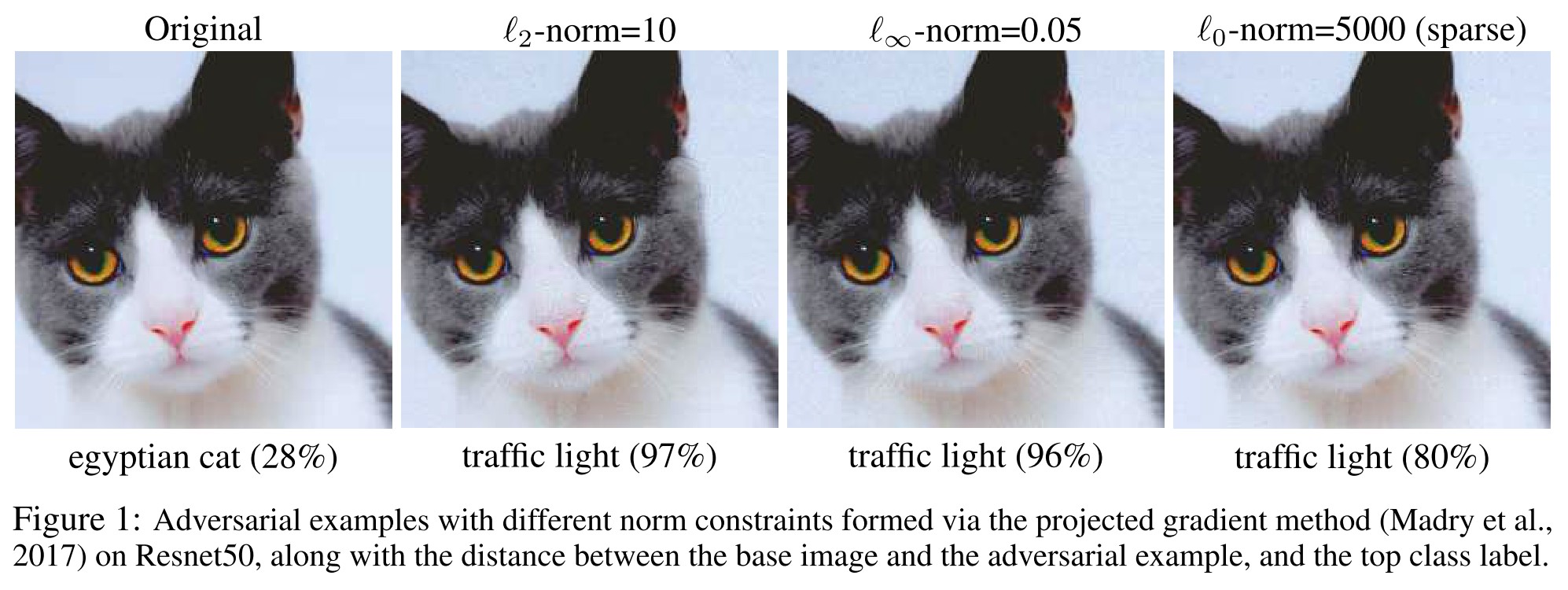
They consider $\ell_p$-norm adversarial examples, and sparse adversarial example, i.e. $\ell_0$-norm adversarial example.

Adversarial Example on the Unit Sphere

The idea is to show that, provided a class of data points takes up enough space, nearly every point in the class lies close to the class boundary.

Definition 2 The $\epsilon$-expansion of a subset $\mathcal{A}\sub \Omega$ with distance metric $d$, denoted $\mathcal{A}(\epsilon, d)$, contains all points that are at most $\epsilon$ units away from $\mathcal{A}$. To be precise

This "for some" is ambiguous.....

Lemma 1 (Isoperimetric inequality). Consider a subset of the sphere $\mathcal{A}\sub\Bbb{S}^{n-1}\sub\R^n$ with normalized measure $\mu_1(\mathcal{A})\ge 1/2$. When using the geodesic metric, the $\epsilon$-expansion $\mathcal{A}(\epsilon)$ is at least as large as the $\epsilon$-expansion of a half sphere.

This lemma indicates that when the $\epsilon$-nerighborhood has an error rate larger than $1/2$, the error set is at least as large as a half sphere expanded with an $\epsilon$ strip.

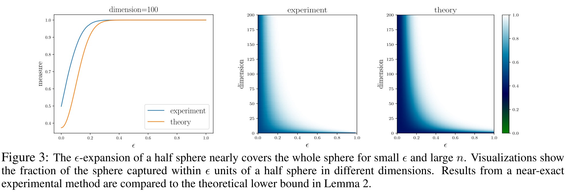
Lemma 2 ($\epsilon$-expansion of half sphere). The geodesic (测地) $\epsilon$-expansion of a half sphere has normalized measure at least

Lemmas 1 and 2 together can be taken to mean that, if a set is not too small, then in high dimensions almost all points on the sphere are reachable within a short jump from that set.

If it's not smaller than a half sphere, is it really appropriate to say that it's not too small? This is ambiguous.

Despite its complex appearance, the result below is a consequence of the (relatively simple) isoperimetric inequality.

Theorem 1 (Existence of Adversarial Examples). Consider a classification problem with $m$ object classes, each distributed over the unit sphere $\Bbb{S}^{n-1}\sub\R^n$ with density functions $\{\rho_c\}_{c=1}^m$. Choose a classifier function $\mathcal{C}:\Bbb{S}^{n-1}\to\{1,2,\dots,m\}$ that partitions the sphere into measurable subsets. Define the following scalar constants:

• Let $V_c$ denote the magnitude of the supremum of $\rho_c$ relative to the uniform density, i.e. $V_c:=s_{n-1}\cdot\sup_x\rho_c(x)$.
• Let $f_c=\mu_c\{x|\mathcal{C}(x)=c\}$ be the fraction of the sphere labeled as $c$ by classifier $\mathcal{C}$.

Choose some class $c$ with $f_c\le\frac{1}{2}$. Sample a random data point $x$ from $\rho_c$. Then with probability at least

one of the following conditions holds:

1. $x$ is misclassified by $\mathcal{C}$, or
2. $x$ admits an $\epsilon$-adversarial example in the geodesic distance

This theorem states that if the semantic classification region of this sphere is smaller than a half sphere, then there is a high probability that any data point inside can reach outside within a small geodesic step of $\epsilon$.

Since for any two points $x$ and $y$ on a sphere,

where $d_{\infty},d_2$ and $d_g$ denote the $\ell_{\infty}$, Euclidean and geodesic distance respectively, therefore, any $\epsilon$-adversarial example in the geodesic metric would also be adversarial in the other two metrics, and the bound in Theorem 1 holds regardless of which of the three metrics we choose.

Adversarial Example on the Unit Cube

In a more typical situation, images will be scaled so that their pixels lie in [0, 1], and data lies inside a high-dimensional hypercube (but, unlike the sphere, data is not confined to its surface).

Fortunately, researchers have been able to derive “algebraic” isoperimetric inequalities that provide lower bounds on the size of the -expansion of sets without identifying the shape that achieves this minimum.

Lemma 3 (Isoperimetric inequality on a cube). Consider a measurable subset of the cube $\mathcal{A}\sub [0,1]^n$, and a $p$-norm distance metric $d_p(x,y)=||x-y||_p,p>0$. Let $\Phi(z)=(2\pi)^{-\frac{1}{2}}\int _{-\infty}^z e^{-t^2/2}dt$, and let $\alpha$ be the scalar that satisfies $\Phi(\alpha)=\text{vol}[\mathcal{A}]$. Then

where $p^*=\min(p,2)$. In particular, if $\text{vol}(\mathcal{A})\ge 1/2$, then we simply have

This lemma states that if the subset occupies more than a half of this space, an $\epsilon$-extension of this subset will occupy nearly the whole space.....?

Using this result, we can show that most data samples in a cube admit adversarial examples, provided the data distribution is not excessively concentrated.

Theorem 2 (Adversarial examples on the cube). Consider a classification problem with $m$ classes, each distributed over the unit hypercube $[0,1]^n$ with density functions $\{\rho_c\}_{c=1}^m$. Choose a classifier function $\mathcal{C}:[0,1]^n\to \{1,2,\dots,m\}$ that partitions the hypercube into disjoint measurable subsets. Define the following scalar constants:

• Let $U_c$ denote the supremum of $\rho_c$.
• Let $f_c$ be the fraction of hypercube partitioned into class $c$ by $\mathcal{C}$.

Choose some class $c$ with $f_c\le \frac{1}{2}$, and select an $\ell_p$-norm with $p>0$. Define $p^*=\min(p,2)$. Sample a random data point $x$ from the class distribution $\rho_c$. Then with probability at least

one of the following conditions holds:

1. $x$ is misclassified by $\mathcal{C}$, or
2. $x$ has an adversarial example $\hat{x}$, with $||x-\hat{x}||_p\le\epsilon$.

For any $p\ge 2$, the bound becomes

It's because $p^*=\min(p,2)$...

As long as the class distribution is not overly concentrated, this bound guarantees adversarial examples with relatively "small" $\epsilon$ relative to a typical vector.

When using the $\ell_{\infty}$-norm, the bound is still equation 5, but the $\ell_{\infty}$ adversarial examples are only interesting if $\epsilon<1$, where the equation 5 becomes vacuous for large $n$.

I think they want to say that when $\epsilon<1$, the equation 5 rapidly reaches 1 as $\epsilon$ reaches 1.

They state that using the tighter bound of equation 2, equation 4 can be replaced with

for $p\ge 2$, where $\hat{\Phi}(z)=\frac{1}{\sqrt{2\pi}}\int_z^{\infty}e^{-t^2/2}dt\ge\frac{1}{\sqrt{2\pi}z}e^{-z^2/2}, z>0$, and $\alpha=\Phi^{-1}(1-f_c)$.

For this bound to be meaningful with $\epsilon<1$, we need $f_c$ to be relatively small, and $\epsilon$ to be roughly $f_c$ or smaller. This is realistic for some problems; ImageNet has 1000 classes, and so $f_c < 10^{−3}$ for at least one class.

Interestingly, under $\ell_{\infty}$-norm attacks, guarantees of adversarial examples are much stronger on the sphere (Section 3) than on the cube.

One can construct examples of sets with $\ell_{\infty}$-expansions that nearly match the behavior of equation 5, and so our theorems in this case are actually quite tight.

I do not get the sense of the last few paragraphs of this section.

Sparse Adversarial Examples

Sparse adversarial examples refer to adversarial examples under the $\ell_0$ metric, i.e.

If a point $x$ has an $\epsilon$-adversarial example in this norm, then it can be perturbed into a different class by modifying at most $\epsilon$ pixels (in this case $\epsilon$ is taken to be a positive integer)

Theorem 2 is fairly tight for p = 1 or 2. However, the bound becomes quite loose for small p, and in particular it fails completely for the important case of p = 0.

Lemma 4 (Isoperimetric inequality on the cube: small $p$). Consider a measurable subset of the cube $\mathcal{A}\sub [0,1]^n$, and a $p$-norm distance metric $d(x,y)=||x-y||_p,p\ge 0$. We have

Theorem 3 (Sparse adversarial examples). Consider the problem setup of Theorem 2. Choose some class with $f_c\le\frac{1}{2}$, and sample a random data point $x$ from the class distribution $\rho_c$. Then with probability at least

one of the following conditions holds:

1. $x$ is misclassified by $\mathcal{C}$, or
2. $x$ can be adversarially perturbed by modifying at most $\epsilon$ pixels, while still remaining in the unit hypercube.

Using this equation, the probability for a uniformly distributed MNIST dataset to have an one-pixel adversarial example is more than 0.8....

I think it's misaligned with the experimental results.

Existence of Adversarial Examples

Tighter bounds can be obtained if we only guarantee that adversarial examples exist for some data points in a class, without bounding the probability of this event.

Theorem 4 (Condition for existence of adversarial examples). Consider the setup of Theorem 2. Choose a class $c$ that occupies a fraction of the cube $f_c<\frac{1}{2}$. Pick an $\ell_p$-norm and set $p^*=\min(p,2)$.

Let $\text{supp}(\rho_c)$ denote the support (支集) of $\rho_c$. Then there is a point $x$ with $\rho_c(x)>0$ that admits an $\epsilon$-adversarial example if

The bound for the case $p=0$ is valid only if $\epsilon\ge\sqrt{n\log 2/2}$.

From wikipedia:

The support of a distribution is the smallest closed interval/set whose complement has probability zero. It may be understood as the points or elements that are actual members of the distribution.

This theorem states that if the distribution distributes large enough, there exists an adversarial example for sure.

When the $\ell_2$-norm is used, the bound becomes

The diameter of the cube is $\sqrt{n}$, and the bound becomes active for

It can be seen that the bound is active whenever the size of the support satisfies

Remarkably, this holds for large $n$ whenever the support of class $c$ is larger than (or contains) a hypercube of side length at least $e^{-\pi}\approx 0.043$.

It seems to say that as long as the data of this class is distributed larger than a small hypercube, there exists an adversarial example.

It is important note, however, that the bound being “active” does not mean there are adversarial examples with a “small” $\epsilon$.

Luckily, if we restrict the adversarial examples to defend to be small, it's still solvable seemingly.

Can We Escape Fundamental Bounds?

There are a number of ways to escape the guarantees of adversarial examples made by Theorems 1-4. One potential escape is for the class density functions to take on extremely large values.

• Unbounded density functions and low-dimensional data manifolds

  In practice, image datasets might lie on low-dimensional manifolds within the cube, and the support of these distributions could have measure zero, making the density function infinite (i.e., $U_c = \infty$)

• Adding a “don’t know” class

  The analysis above assumes the classifier assigns a label to every point in the cube. If a classifier has the ability to say “I don’t know,” rather than assign a label to every input, then the region of the cube that is assigned class labels might be very small, and adversarial examples could be escaped even if the other assumptions of Theorem 4 are satisfied. In this case, it would still be easy for the adversary to degrade classifier performance by perturbing images into the “don’t know” class.

  It does not solve the problem.....

• Feature squeezing

  If decreasing the dimensionality of data does not lead to substantially increased values for $U_c$ (we see in Section 8 that this is a reasonable assumption) or loss in accuracy (a stronger assumption), measuring data in lower dimensions could increase robustness.

  It seems to me that $U_c$ is better to be larger, so the probability lower bound is smaller.....

• Computational hardness

  It may be computationally hard to craft adversarial examples because of local flatness of the classification function, obscurity of the classifier function, or other computational difficulties.

  This is the defense of gradient masking....But it does not solve the problem either.

Experiments

It is commonly thought that high-dimensional classifiers are more susceptible to adversarial examples than low-dimensional classifiers. This perception is partially motivated by the observation that classifiers on highresolution image distributions like ImageNet are more easily fooled than low resolution classifiers on MNIST.

We will see below that high dimensional distributions may be more concentrated than their low-dimensional counterparts.

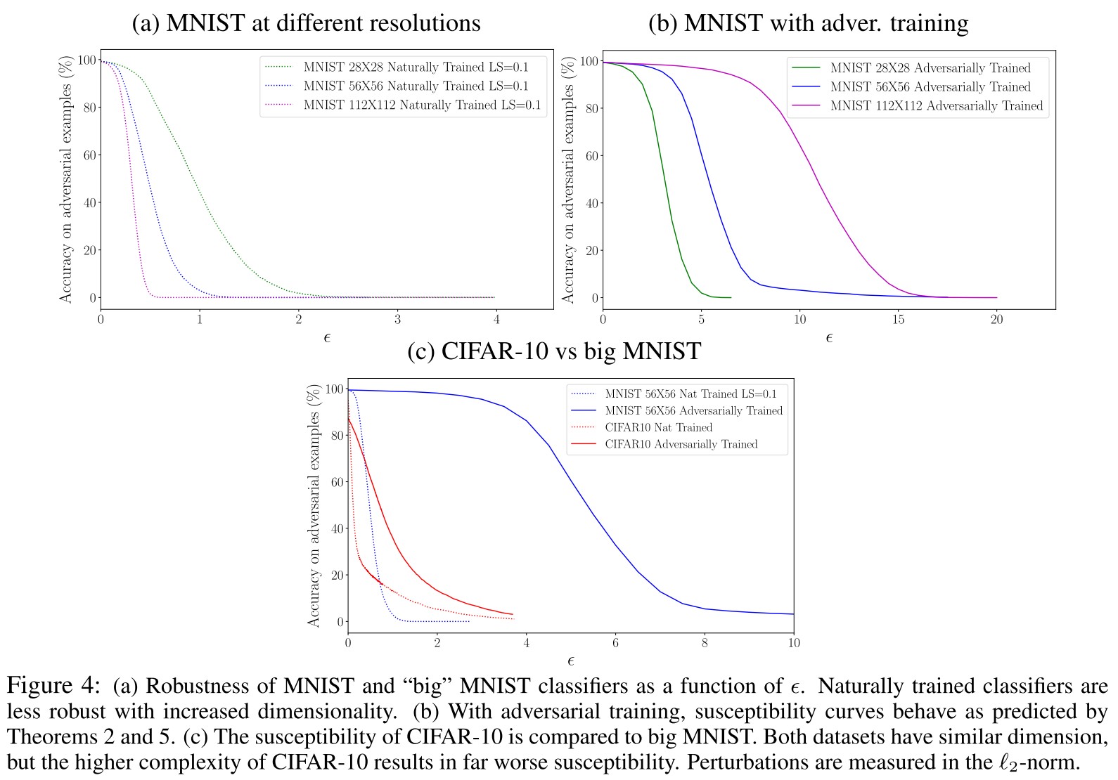
The theorem below shows that these fundamental limits do not depend in a non-trivial way on the dimensionality of the images in big MNIST, and so the relationship between dimensionality and susceptibility in Figure 4a results from the weakness of the training process.

Theorem 5 Suppose $\epsilon$ and $p$ are such that, for all MNIST classifiers, a random image from class $c$ has an $\epsilon$-adversarial example (in the $\ell_2$-norm) with probability at least $p$. Then for all classifiers on b-MNIST, with integer $b\ge 1$, a random image from $c$ has a $b\epsilon$-adversarial example with probability at least $p$.

Likewise, if all $b$-MNIST classifiers have $b\epsilon$-adversarial examples with probability $p$ for some $b\ge 1$, then all classifiers on the original MNIST distribution have $\epsilon$-adversarial examples with probability $p$.

They want to state that the vulnerability stems from data distribution and it is trivially related to dimensionality.

Theorem 5 predicts that the perturbation needed to fool all 56 × 56 classifiers is twice that needed to fool all 28 × 28 classifiers. This is reasonable since the $\ell_2$-norm of a 56 × 56 image is twice that of its 28 × 28 counterpart.

As shown in Figure 4b:

As predicted by Theorem 5, the 112×112 classifier curve is twice as wide as the 56×56 curve, which in turn is twice as wide as the 28×28 curve. In addition, we see the kind of “phase transition” behavior predicted by Theorem 2, in which the classifier suddenly changes from being highly robust to being highly susceptible as passes a critical threshold.

For these reasons, it is reasonable to suspect that the adversarially trained classifiers in Figure 4b are operating near the fundamental limit predicted by Theorem 2.

This is a theoretically backup for adversarial training.....

But then why are high-dimensional classifiers so easy to fool?

The smallest possible value of $U_c$ is 1, which only occurs when images are “spread out” with uniform, uncorrelated pixels. In contrast, adjacent pixels in MNIST (and especially big MNIST) are very highly correlated, and images are concentrated near simple, low-dimensional manifolds, resulting in highly concentrated image classes with large $U_c$.

$U_c$ is defined as the supremum of a density function $\rho_c$, how can it be larger than 1?

As shown in Figure 4c:

We can reduce $U_c$ and dramatically increase susceptibility by choosing a more “spread out” dataset, like CIFAR-10, in which adjacent pixels are less strongly correlated and images appear to concentrate near complex, higher-dimensional manifolds.

The former problem lives in 3136 dimensions, while the latter lives in 3072, and both have 10 classes. Despite the structural similarities between these problems, the decreased concentration of CIFAR-10 results in vastly more susceptibility to attacks, regardless of whether adversarial training is used.

Informally, the concentration limit $U_c$ can be interpreted as a measure of image complexity. Image classes with smaller $U_c$ are likely concentrated near high-dimensional complex manifolds, have more intra-class variation, and thus more apparent complexity.

An informal interpretation of Theorem 2 is that “high complexity” image classes are fundamentally more susceptible to adversarial examples.

The interpretation is reasonable, but the meaning of $U_c$ seems to be ambiguous.

Are Adversarial Examples Inevitable?

The question of whether adversarial examples are inevitable is an ill-posed one. Clearly, any classification problem has a fundamental limit on robustness to adversarial attacks that cannot be escaped by any classifier. However, we have seen that these limits depend not only on fundamental properties of the dataset, but also on the strength of the adversary and the metric used to measure perturbations. This paper provides a characterization of these limits and how they depend on properties of the data distribution. Unfortunately, it is impossible to know the exact properties of real-world image distributions or the resulting fundamental limits of adversarial training for specific datasets. However, the analysis and experiments in this paper suggest that, especially for complex image classes in high-dimensional spaces, these limits may be far worse than our intuition tells us.

Inspirations

They give a comprehensive analysis of the existence of adversarial examples. They point out that the higher adversarial vulnerability of higher dimensional data stems from the training process and use adversarially trained models demonstrate that fundamentally the adversarial perturbation required increases as dimension increases.

Thus, fundamentally, the adversarial vulnerability stems from data distribution, i.e. the concentration of data points from each class.

This explains why CIFAR-10 is much more difficult than MNIST for adversarial robustness.