Orthogonal Convolution

By LI Haoyang 2020.10.19

Content

OCNN

Paper: https://arxiv.org/abs/1911.12207v1

Code: https://github.com/samaonline/Orthogonal-Convolutional-Neural-Networks

Jiayun Wang Yubei Chen Rudrasis Chakraborty Stella X. Yu. Orthogonal Convolutional Neural Networks. CVPR 2020

Kernel Orthogonality VS Orthogonal CNN

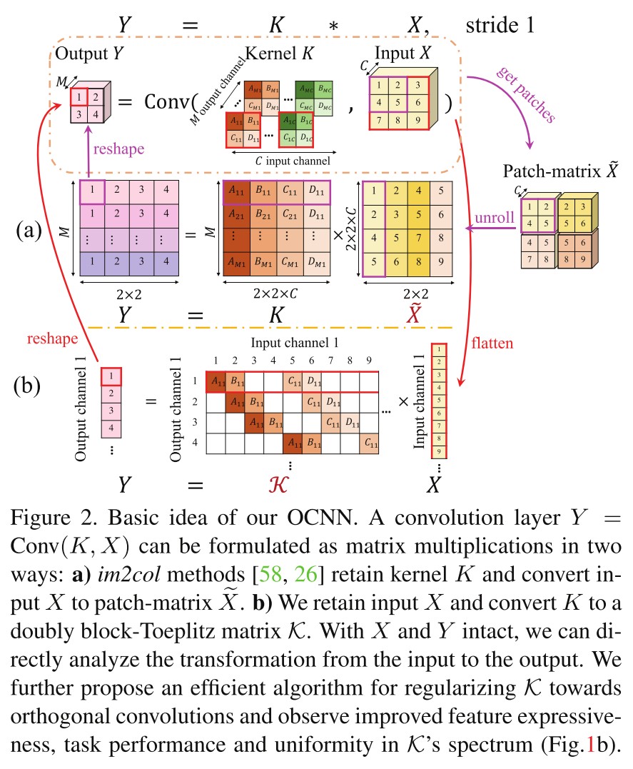
For a convolution layer $Y=Conv(K,X)$, the differences are:

• Kernel orthogonality

  It views the convolution as multiplication between the kernel matrix $K$ and the im2col matrix $\tilde{X}$, i.e. $Y=K\tilde{X}$.

  The orthogonality is enforced by penalizing the disparity between the Gram matrix of kernel $K$ and the identity matrix, i.e. $||KK^T-I||$.

• Orthogonal convolution

  It keeps the input $X$ and the output $Y$ intact by connecting them with a doubly block-Toeplitz (DBT) matrix $\cal{K}$ of filter $K$, i.e. $Y=\mathcal{K}X$ and enforces the orthogonality of $\mathcal{K}$ directly.

Orthogonal Convolution

Convolution as a matrix-vector multiplication

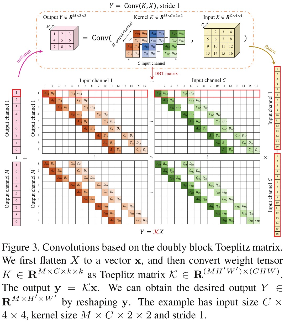
For a convolution layer with input tensor $X\in \Bbb{R}^{C\times H\times W}$ and kernel $K\in \Bbb{R}^{M\times C\times k\times k}$, which can be viewed as $M$ different filters .i.e. $\{K_i\in \Bbb{R}^{C\times k\times k}\}$, the convolution's output tensor is $Y=Conv(K,X)$, where $Y\in \Bbb{R}^{M\times H^{'}\times W^{'}}$. Since convolution is linear, it can be rewritten in a matrix-vector form:

In which, $y$ and $x$ are the flattened version of $Y$ and $X$.

Each row of $\cal{K}$ has non-zero entries corresponding to a particular filter $K_i$, it can be constructed as a doubly block-Toeplitz (DBT) matrix $\mathcal{K}\in\Bbb{R}^{(MH^{'}W^{'})\times (CHW)}$ from kernel tensor $K\in \Bbb{R}^{M\times C\times k\times k}$.

Convolutional orthogonality

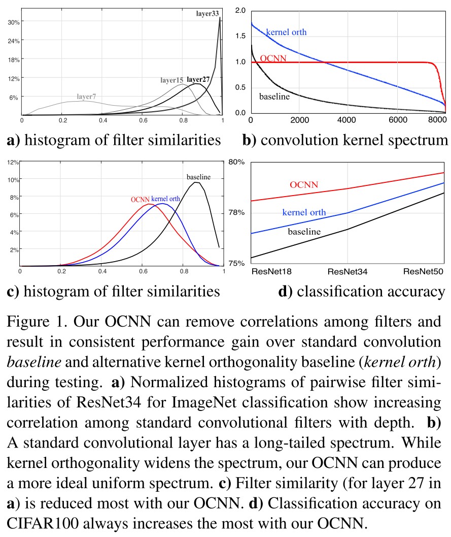
To increase the orthogonality of convolution, their approach is to regularize the spectrum of $\cal{K}$ to be uniform.

The uniform spectrum requires a row orthogonal convolution for a fat matrix case ($MH^{'}W^{'}\le CHW$) and a column orthogonal convolution for a tall matrix case ($MH^{'}W^{'}\ge CHW$) where $\cal{K}$ is a normalized frame and preserves the norm.

• Row Orthogonality

  Each row of $\cal{K}$ is a flattened filter $K_i$, denoted as $\mathcal{K}_{ih^{'}w^{'},\cdot \in\Bbb{R}^{CHW}}$.

  The row orthogonality condition is:

  $$\left<\mathcal{K}_{ih^{'}_1w_1^{'},\cdot},\mathcal{K}_{jh_2^{'}w_2^{'},\cdot}\right>=\begin{cases} 1,(i,h_1^{'},w_1^{'})=(j,h_2^{'},w_2^{'})\\ 0, otherwise \end{cases}$$

  For the patches whose flattened version do not overlap, the corresponding rows are naturally orthogonal, i.e. those of $|h_1-h_2|\ge k$ or $|w_1-w_2|\ge k$.

  By implementation, they can utilize the spatial symmetry to vary $i,j,h_2,w_2$ only, with fixed $h_1,w_1$. The region to check orthogonality can be realized by the original convolution with padding: $P=\left[\frac{k-1}{S}\right]\cdot S$, where the $S$ denotes the stride.

  

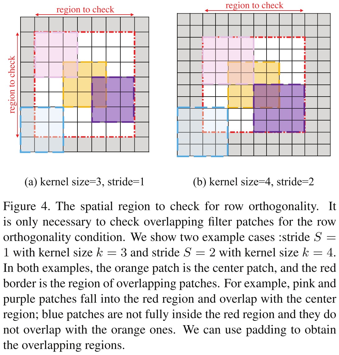
  Then the condition is equivalent to the following self-convolution:

  $$Conv(K,K,padding=P,stride=S)=I_{r0}$$

  In which, $I_{r0}\in \Bbb{R}^{M\times M\times (2P/S+1)\times(2P/S+1)}$ is tensor who has zero entries except for center $M\times M$ entries as an identity matrix.

• Column Orthogonality

  One can obtain a column $\cal{K}_{\cdot,ihw}$ of $\cal{K}$ by the following equation:

  $$\mathcal{K}_{\cdot,ihw}=\mathcal{K}\bold{e}_{ihw}=Reshape(Conv(K,E_{i,h,w}))$$

  In which, $\bold{e}_{ihw}\in\Bbb{R}^{CHW}$ is the flattened vector of an artificial input $E_{i,h,w}\in \Bbb{R}^{C\times H\times W}$, who has all zero except an 1 entry at $(i,h,w)$.

  The column orthogonality condition is:

  $$\left<\mathcal{K}_{\cdot,ih_1w_1},\mathcal{K}_{\cdot,jh_2,w_2}\right>=\begin{cases} 1,(i,h_1,w_1)=(j,h_2,w_2)\\ 0,otherwise \end{cases}$$

  There is also a simpler equivalent of this condition (with stride 1):

  $$Conv(K^{T},K^{T},padding=k-1,stride=1)=I_{c0}$$

  In which, $K^{T}$ is the input-output transposed $K$, i.e. $K^T\in \Bbb{R}^{C\times M\times k\times k}$, $I_{c0}\in \Bbb{R}^{C\times C\times (2k-1)\times (2k-1)}$ has all zeros except for the center $C\times C$ entries as an identity matrix.

The kernel row and column orthogonality is a special case of the conditions above when the stride is $k$:

In which, $I_{r0}\in\Bbb{R}^{M\times M\times 1\times 1}$ and $I_{c0}\in\Bbb{R}^{C\times C\times C\times 1\times 1}$ are identity matrices.

This condition is clearly necessary but not sufficient for the orthogonal convolution conditions.

Given the following Lemma:

Lemma 1. The row orthogonality and column orthogonality are equivalent in the MSE sense, i.e. $||\mathcal{K}\mathcal{K}^T-I||_F^2=||\mathcal{K}\mathcal{K}^T-I^{'}||_{F}^2+U$, where $U$ is a constant.

The finally loss with regularization is:

Performance

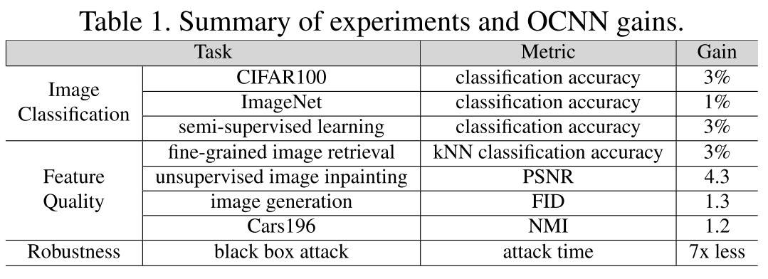
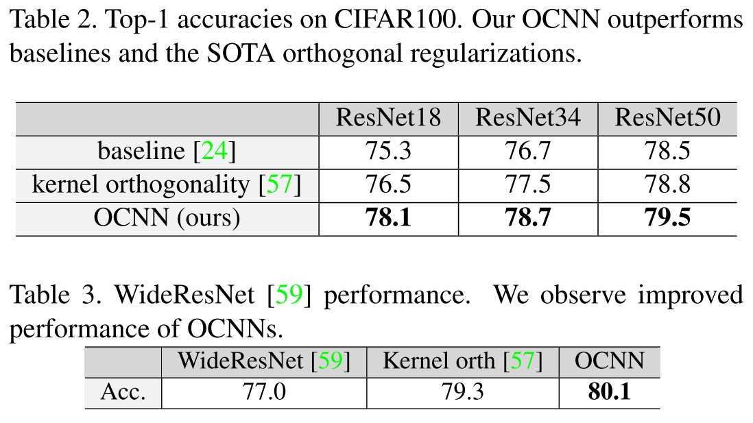
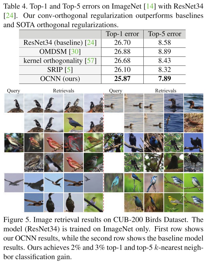
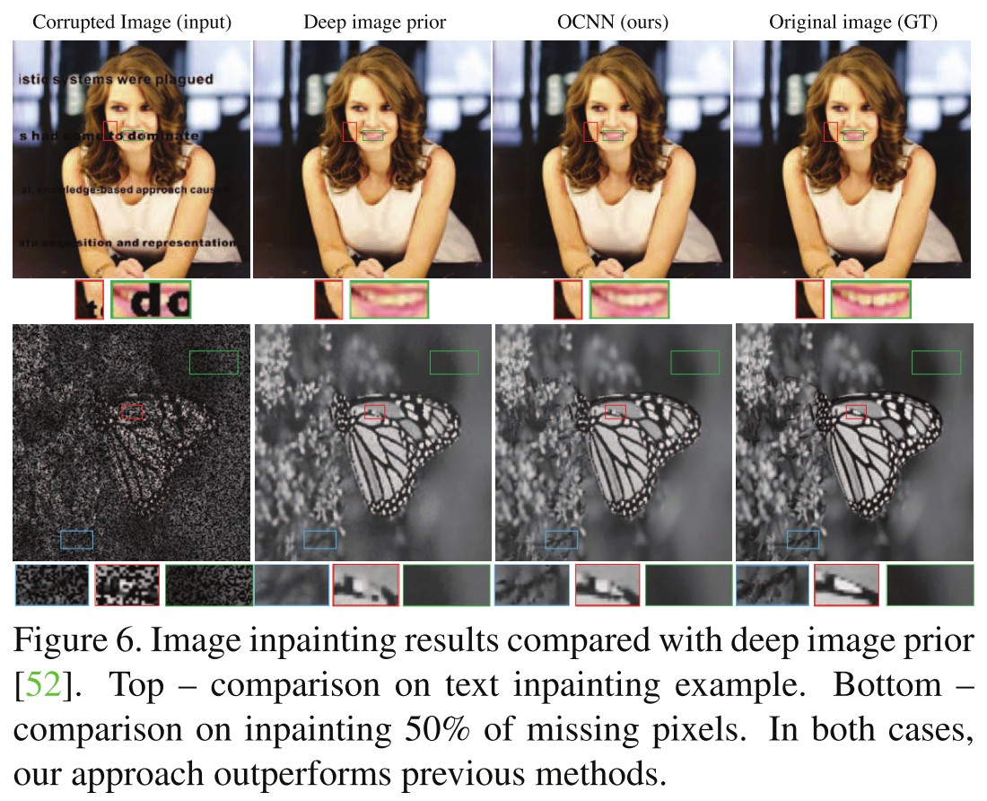
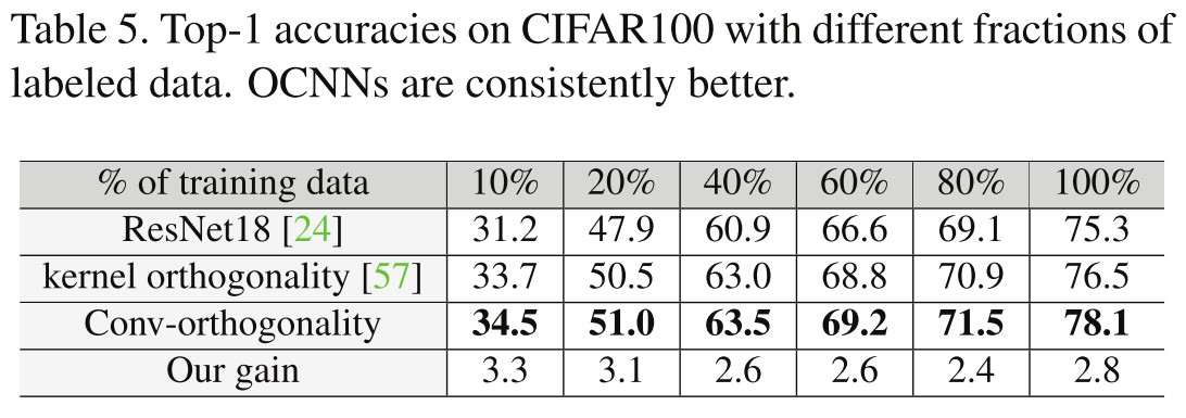
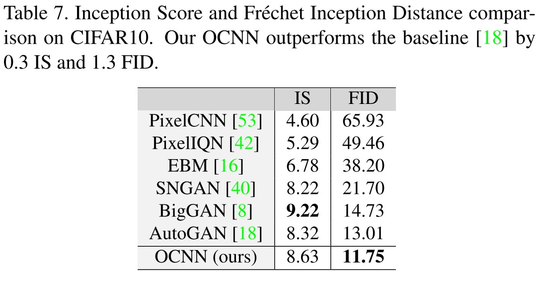
Robustness under Adversarial Attack

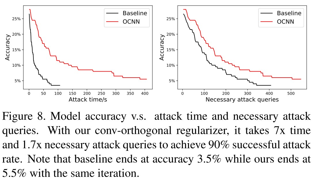
The uniform spectrum of $\cal{K}$ makes each convolution layer approximately an 1-Lipschitz function. Given a small perturbation to input, $\Delta x$, the change of output $\Delta y$ is bounded to be low.

Inspirations

It sounds very natural that a more orthogonal set of kernels captures a more diverse set of features, and a more diverse set of features helps with the performance of models. In another perspective, orthogonal kernels have limited power, i.e. stabler gradients propagated during training, thus a more smooth and stable training is acquired.

However, by restricting strong orthogonality, the transformation done by the linear part of each layer is restricted to rotation in the space, which seems to be a little to restrictive for the model to work at its best.

Since the Lipshitz bound is lowered for each layer, it's rational for it to be more robust to adversarial attacks, but the resistance reported seems not that competitive with adversarial training.