A simple survey of object detection

By Haoyang Li 2020.9.23 ~ 2020.9.30

Conclusion before everything

Feelings

• PASCAL VOC has been conquered (the latest mAP reaches 0.9+);
• MS COCO has challenged existing methods with a new metric (although might not be reasonable);
• One-stage gets speed, two-stage gets accuracy and they are merging;
• End-to-end is preferred;
• A powerful backbone is very useful;
• New structures are coming!

Thoughts

Besides the desire for better accuracy and higher speed, there are few thoughts unsolved in my mind:

• Is it possible to put method into use without further training?. Most methods adopt a combination of pre-trained feature extractor and a customized network. The pre-trained backbone is really powerful, but it does not cover every class of objects in real life, which causes customized re-fine-tuning is required for practical use.
• Does current metric really reflects the real situation? As mentioned by the author of YOLO in the tech report of YOLOv3, the extreme challenging metric used by MS COCO is not quite reasonable. But it seems that no discussion about it appears in other paper.
• What is the definition of object? The definition of object itself seriously introduces the problem of overlap. If face is an object to detect, how about eyes, nose and mouth? If eye is an object to detect, how about iris, eyelid and pupil? Most objects themselves are divisible and combinable. It may be very useful if the detection system allows customized definition for objects without re-training.
• Is there better way to deal with multi-scale? Since the publish of FPN, resolving the problem of multi-scale with the fusion of feature maps in different layers quickly prevails. But this process actually introduces a prior of feature maps. It pre-defines the ratio between the smallest object and biggest object. The authors of the newest end-to-end method, DETR, have not considered the problem of multi-scale yet and they also encourage the use of multiple feature maps while trying to eliminate other priors like anchors, centers, etc. Is there a method to eliminate the prior of feature maps?
• Is box the best representation of the location and size of an object? Human never locate an object with boxes as you can test with yourself. To locate an object with a box is very intuitive and handy for algorithms, but it does not work well with rotated objects, thus many researches have been done to expand the idea of bounding box into angled bounding box. CornerNet, CenterNet and RepPoints have done some work on new representations of object location, but still constrained by the idea of bounding box. Is there a better representation?
• Do we really need the task of object detection? The very refinement of bounding box makes the task of object detection itself redundant compared to semantic segmentation. If an object is detected with its accurate border from the background, then what's the difference between object detection and semantic segmentation? It makes object detection a coarse and faster semantic segmentation (or they are fundamentally the same task with different emphasis). So why not use a coarse and fast version of semantic segmentation method to do the trick?
• Is it possible to train, test and deploy an object detection model with a personal laptop? The current methods all require pre-trained weights, which is centered and controlled by authorities, huge datasets, which is not even possible to store in personal laptop, and powerful hardwares to train days even weeks. Go along with this direction of development, huge companies even nations will be the only entities to train a network. By then, the community will be a solo stage where performers are the raters, which is not the ideal future of research in every researcher's mind.

Task description

Given an image, predict each object's location (x and y position), size (height and width), class (what it is) and confidence (how confident).

Goal:

• Faster : higher frame per second
• More precision: higher mAP (mean average precision)
• More recall: detect every objects that should be detected

Datasets

PASCAL VOC 2005~2012

Website: http://host.robots.ox.ac.uk/pascal/VOC/

VOC 2005

Only 4 classes: bicycles, cars, motorbikes, people. Train/validation/test: 1578 images containing 2209 annotated objects.

VOC 2012

20 classes. The train/val data has 11,530 images containing 27,450 ROI annotated objects and 6,929 segmentations.

Detection task

1- Task

For each of the twenty classes predict the bounding boxes of each object of that class in a test image (if any). Each bounding box should be output with an associated real-valued confidence of the detection so that a precision/recall curve can be drawn....

4- Evaluation

...To be considered a correct detection, the area of overlap ao between the predicted bounding box Bp and ground truth bounding box Bgt must exceed 50% by the formula $a_o=\frac{area(B_p\cap{B_{gt}})}{area(B_p\cup{B_{gt}})}$ ...

Calculation of AP

3.4.1 Average Precision (AP)

The computation of the average precision (AP) measure was changed in 2010 to improve precision and ability to measure differences between methods with low AP. It is computed as follows:

1. Compute a version of the measured precision/recall curve with precision monotonically decreasing, by setting the precision for recall r to the maximum precision obtained for any recall r ′ ≥ r.
2. Compute the AP as the area under this curve by numerical integration. No approximation is involved since the curve is piecewise constant.

MS COCO 2014

Website: https://cocodataset.org/

The 2014 release contains 82,783 training, 40,504 validation, and 40,775 testing images (approximately 1/2 train, 1/4 val, and 1/4 test). There are nearly 270k segmented people and a total of 886k segmented object instances in the 2014 train+val data alone. The cumulative 2015 release will contain a total of 165,482 train, 81,208 val, and 81,434 test images.

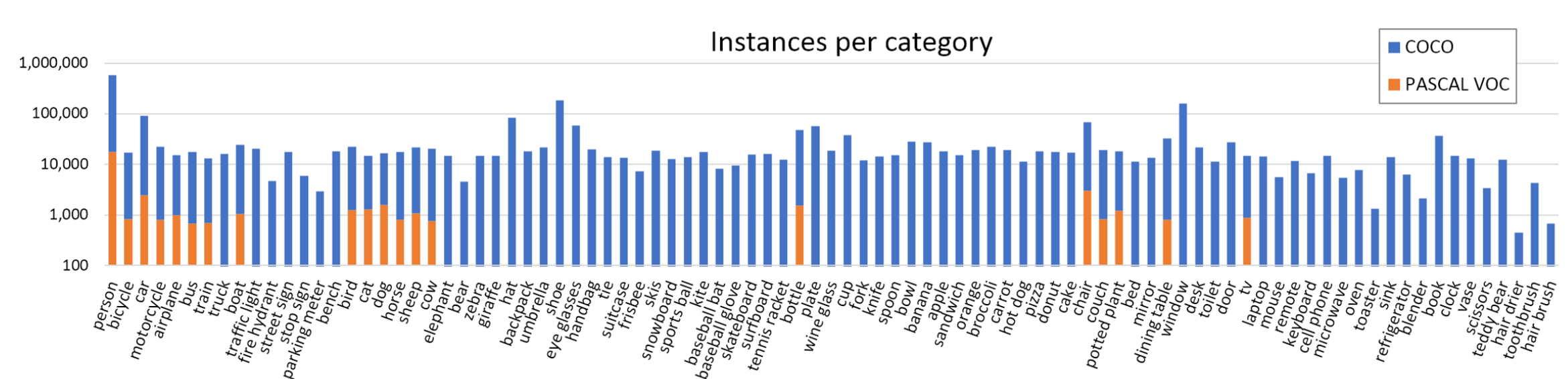
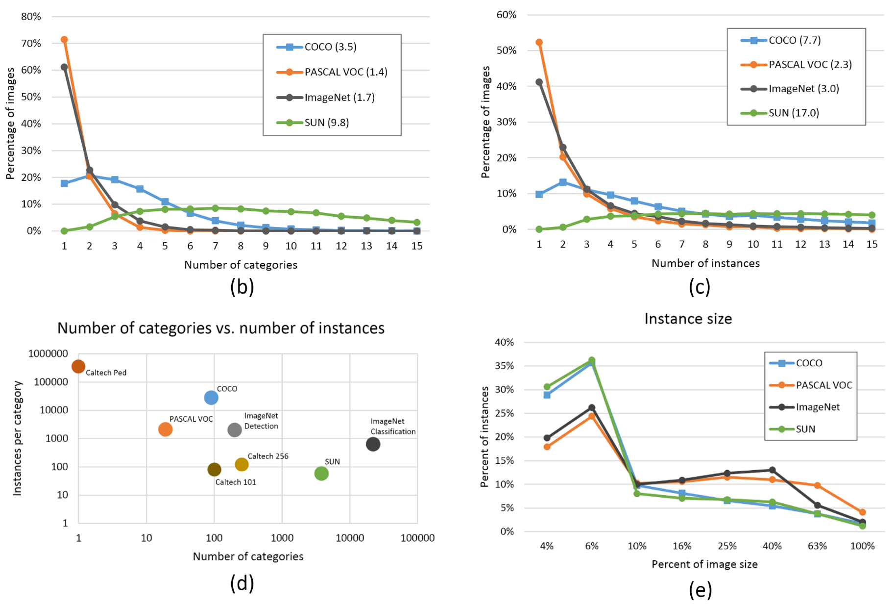
Features

• More images
• More non-iconic images (objects in natural context)
• More smaller objects
• More objects per image
• More categories of objects

Statistics

Calculation of AP

AP - average over 10 IoU thresholds (0.5:0.05:0.95) (primary challenge metric)

AP@0.5 - average precision under IoU of 0.5 (PASCAL VOC metric)

AP@0.75 - average precision under IoU of 0.75 (strict metric)

AP_small, AP_medium, AP_large - small < 322 < medium < 962 < large (average precision for objects in different scales)

Major Models

Zhengxia Zou, Zhenwei Shi, Yuhong Guo and Jieping Ye. Object Detection in 20 Years: A Survey. 2019. arXiv:1905.05055

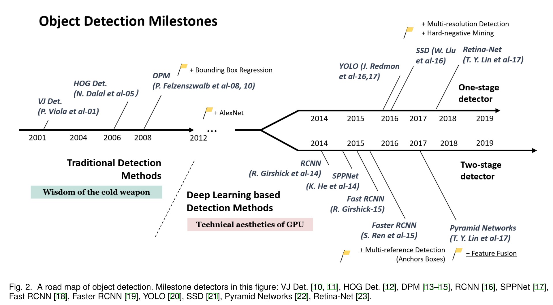
From explicit, disjoint modules to implicit end-to-end module:

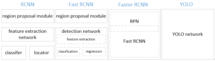
Generally, the two-stage methods are better in terms of average precision, while the one-stage methods have advantages in speed, making the latter more practical and more popular in industry.

Paradigms

A typical pipeline of current methods is as follows:

But actually the first stage, region proposal, of two-stage methods is much like a detector with fewer accuaracy, therefore, a two-stage method can be illustrated as a cascade of a coarse one-stage method and a fine-grained one-stage method.

Two-stage

Reference: Faster R-CNN

One-stage

Reference: YOLOv3

R-CNN family

A typical two-stage method family. The basic pipeline consists of two stages:

1. Region proposal
2. Classify and locate

R-CNN - CVPR 2014

The original R-CNN first introduced CNN into the task of object detection

R. Girshick, J. Donahue, T. Darrell and J. Malik, "Rich Feature Hierarchies for Accurate Object Detection and Semantic Segmentation," 2014 IEEE Conference on Computer Vision and Pattern Recognition, Columbus, OH, 2014, pp. 580-587, doi: 10.1109/CVPR.2014.81.

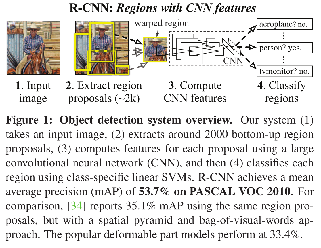
The strategy is explicit:

1. Extract region proposals from input image (using Selective Search)
2. Compute CNN features for each region (using pre-trained CNN)
3. Classify features for each region (using SVM), regress the bounding boxes for each region
4. Use non-maximum suppression to exclude extra bounding boxes

Drawbacks:

1. Training is a multi-stage pipeline
2. Training is expensive in space and time
3. Object detection is slow

Fast R-CNN - ICCV 2015

Code: https://github.com/rbgirshick/fast-rcnn

Based on R-CNN, it reduces the number of inferences conducted by CNN feature extractors to accelerate the whole process.

R. Girshick, “Fast R-CNN,” in IEEE International Conference on Computer Vision (ICCV), 2015.

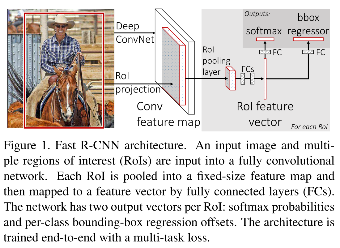
The strategy is explicit:

1. Compute for a feature map over the input image using CNN
2. Extract region proposals from feature map (using Selective Search ?)
3. For each object, extract a RoI out of the feature map and apply RoI pooling, fc layers to get a RoI feature vector
4. For each RoI feature vector, draw two branches: one for the predictions of K object classes plus background; another for the regression of bounding boxes for K object classes (regress for four real values $(r,c, h, w)$, top-left corner and size)
5. Use non-maximum suppression to exclude extra bounding boxes (?)

RoI max pooling works by dividing the h × w RoI window into an H × W grid of sub-windows of approximate size h/H ×w/W and then max-pooling the values in each sub-window into the corresponding output grid cell

Classification branch predicts $p=(p_0,...,p_K)$ over K+1 categories.

Regression branch predicts bounding-box regression offsets for each of K categories as:

The loss is calculated as:

In which, $L_{cls}(p,u)=-logp_u$ is log loss for true class u. For a true bounding-box targets $(v_x,v_y,v_w,v_h)$ and a predicted tuple $(t_x^k,t_y^k,t_w^k,t_h^k)$, the location loss is calculated as:

Faster R-CNN - NIPS 2015 / TPAMI 2015

Code: https://github.com/rbgirshick/py-faster-rcnn

Good illustration: 一文读懂Faster RCNN

Proposed a region proposal network to replace Selective Search in Fast R-CNN to drastically reduce the inference time.

It reaches a speed of 5 fps on a GPU.

Ren S , He K , Girshick R , et al. Faster R-CNN: Towards Real-Time Object Detection with Region Proposal Networks[J]. IEEE Transactions on Pattern Analysis and Machine Intelligence, 2015, 39(6).

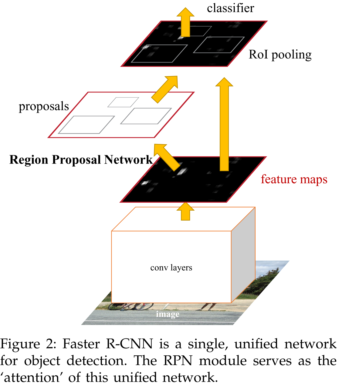
Overall strategy:

1. Compute for a feature map over the input image using CNN
2. Train a region proposal network and a Fast R-CNN module in a 4-step manner
3. Infer from proposals using Fast R-CNN for final results

Region Proposal Network

The overall process of RPN is as:

1. Generate dense anchor boxes (9 anchor boxes for each point on feature map)
2. Binary classify these anchor boxes (positive or negative)
3. Regress for a set of modification values ( $t$ in bounding-box coordinates parameterization)
4. Apply modification values to positive anchors to generate proposals

Structure

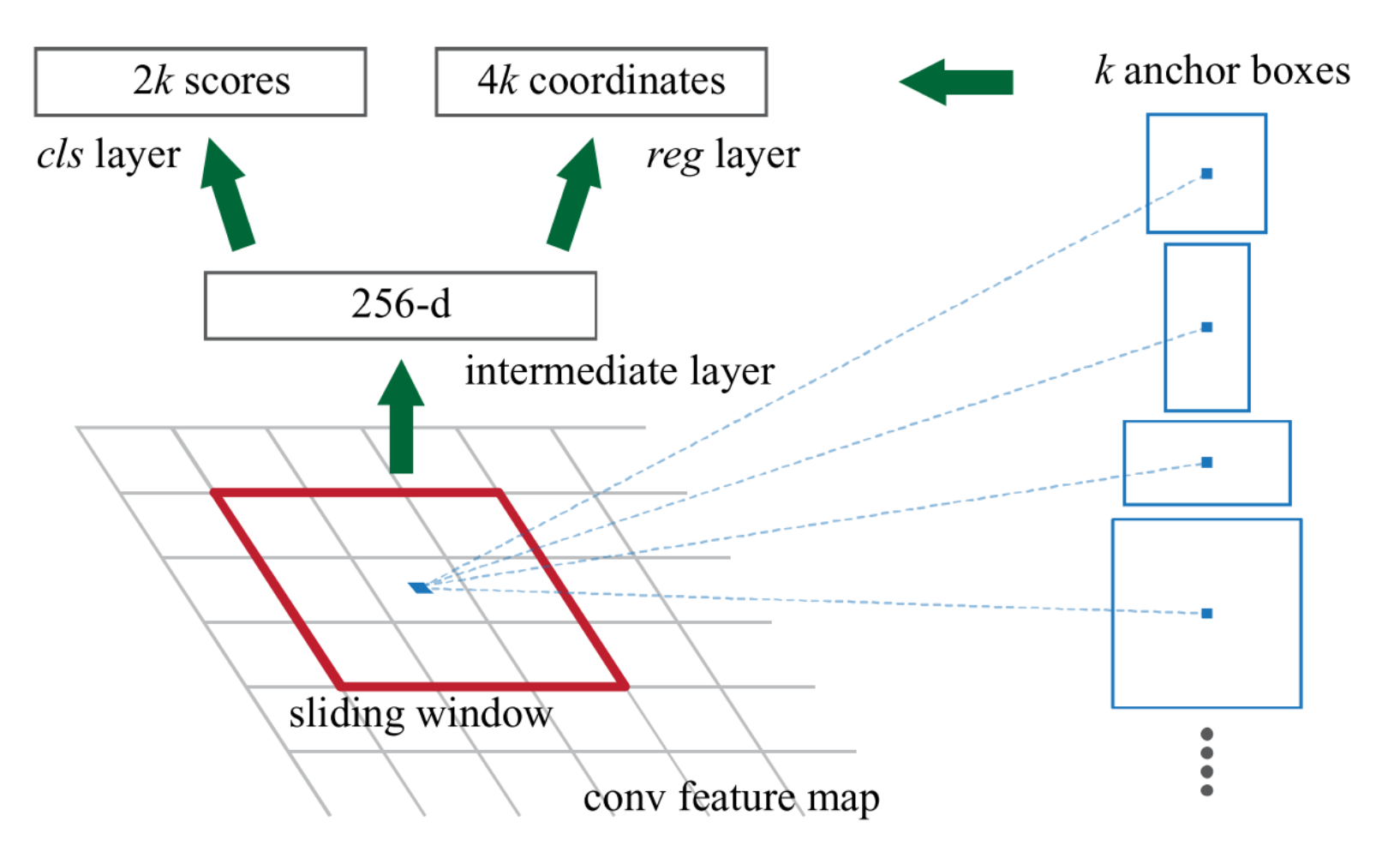
On a feature map, $k$ anchor boxes will be generated for a sliding window, yielding $2k$ scores representing the objectness (positive or negative) of $k$ anchor boxes and $4k$ coordinates representing the location (four values) of $k$ anchor boxes. The pyramid of anchor boxes copes with multi-scale objects as the pyramid of images and the pyramid of filters does.

Loss

The loss function is defined as:

In which, $p_i$ is the predicted probability of anchor $i$ being an object. The ground truth $p_i^*$ is 1 if the anchor is positive and 0 otherwise.

We assign a positive label to two kinds of anchors:

(i) the anchor/anchors with the highest Intersection-over-Union (IoU) overlap with a ground-truth box

(ii) an anchor that has an IoU overlap higher than 0.7 with any ground-truth box.

$t_i$ is a vector representing the 4 parameterized coordinates of the predicted bounding-box, and $t_i^*$ is that of ground truth.

In our current implementation (as in the released code), the $cls$ term in Eqn.(1) is normalized by the mini-batch size (i.e., $N_{cls}$ = 256) and the $reg$ term is normalized by the number of anchor locations (i.e., $N_{reg}$∼ 2, 400). By default we set $\lambda$= 10, and thus both $cls$ and $reg$ terms are roughly equally weighted.

Bounding-box coordinates parameterization

From original $(x, y,w, h)$ to parameterized $(t_x, t_y,t_w,t_h)$ :

This can be thought of as bounding-box regression from an anchor box to a nearby ground-truth box.

4-Step alternating training

1. Train the RPN (using ImageNet-pre-trained model) alone
2. Train a seperate detection network by Fast R-CNN, using the proposals generated by step-1 RPN
3. Use the detector network to initialize RPN training and only fine-tune the layers unique to RPN.
4. Keep the shared convolutional layers fixed and fine-tune the unique layers of Fast R-CNN.

Non-maximum suppression is utilized when RPN generates RoI images for the training of Fast R-CNN, and only a limited and balanced set of RoI positive and negative images are further used for training.

YOLO family and its one-stage companies

YOLOv1 - CVPR 2016

Website: https://pjreddie.com/darknet/yolo/

You only look once, end-to-end object detection network

Joseph Redmon, Santosh Divvala, Ross Girshick, Ali Farhadi, You Only Look Once: Unified, Real-Time Object Detection

Features

• Extremely fast (45 fps+), fair mPA
• Highly generizable
• Frame object detection as a regression problem
• More localization errors, less false positives
• Struggles with small or clustered objects
• Struggles with new objects

Structure

The input image is divided into $S\times S$ grids, for each grid, it predicts $B$ bounding boxes, and for each bounding boxes, it predicts $5$ corresponding values $x, y, w, h, confidence$. Besides, it also predicts $C$ conditional class probabilities for each grid. Thus the output is an $S \times S \times (B * 5 + C)$ tensor.

The location ($x,y$) is relative to the bounds of the grid cell, the size ($w,h$) is relative to the size of image.

The confidence for each bounding box is calculated as $\begin{cases} Pr(Object)*IOU_{pred}^{truth},obj\\ 0, noobj \end{cases}$

The $i$th conditional probability for each grid is calculated as $Pr(Class_i|Object)$ .

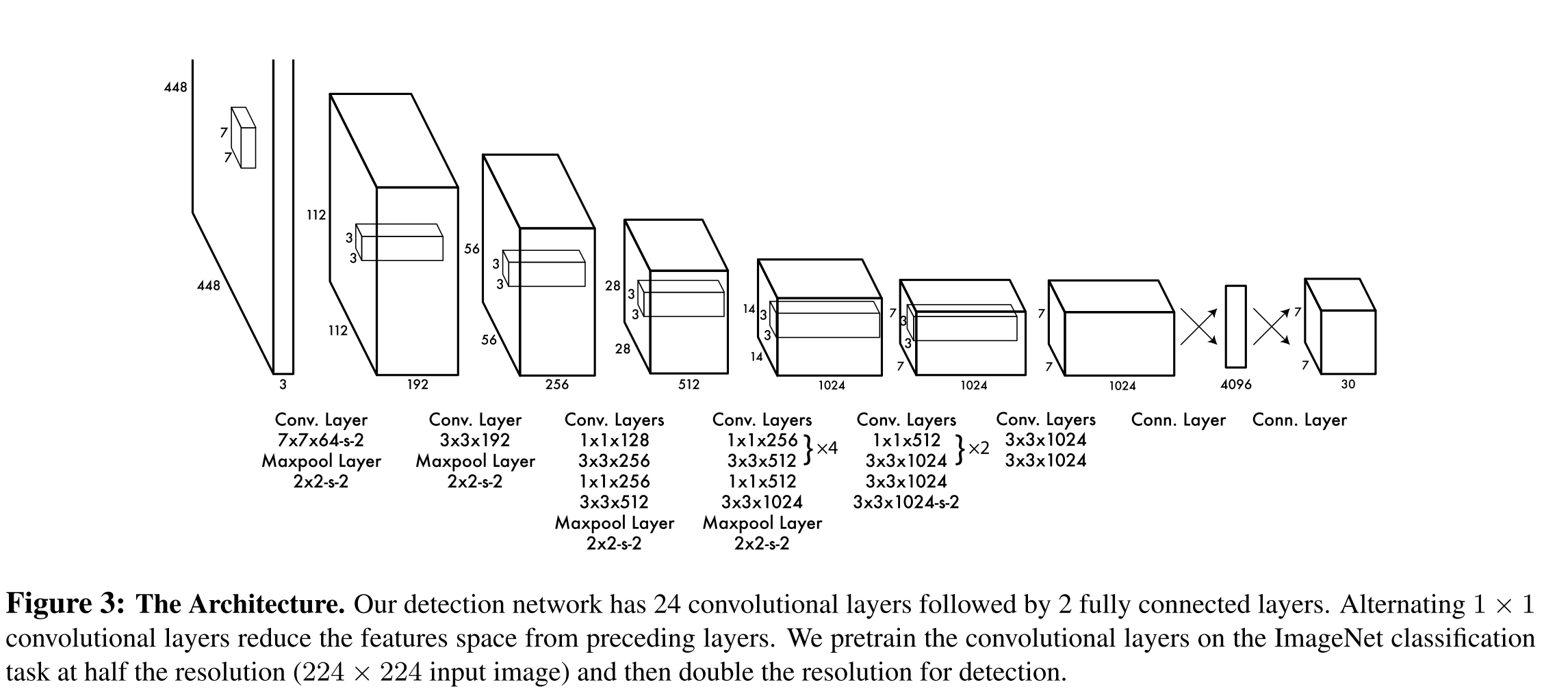
Divide image into $7 \times 7$ grids, and predict $2$ bounding boxes for each grid on $20$ classes of Pascal VOC dataset, it results the output tensor of size $7 \times 7 \times 30$. The structure of net is shown above.

Loss

Predict location (x,y), size (w,h), existence (p_obj) and class (p_class) in an end-to-end form.

Loss for location:

Loss for size:

Loss for existence:

Loss for class:

Sum them up for the final loss function.

$\mathbb{1}_i^{obj}$ denotes if the $i$ th cell contains object; $\mathbb{1}_{ij}^{obj}$ denotes if the $j$th bounding box in $i$th cell is responsible for the prediction (contains the center of object).

VOC 2007 error analysis

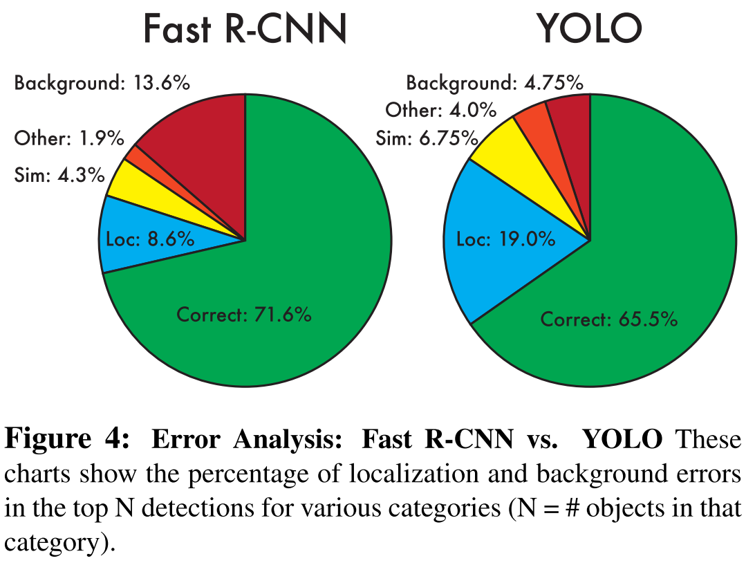
Definition of each type of error:

• Correct: correct class and IOU > 0.5 (true positive)
• Localization: correct class, 0.1 < IOU < 0.5
• Similar: class is similar, IOU > 0.1
• Other: class is wrong, IOU > 0.1
• Background: IOU < 0.1 for any object (false positive)

YOLOv2 - CVPR 2017

Website: http://pjreddie.com/yolo9000/

YOLO with improvements

J. Redmon and A. Farhadi, "YOLO9000: Better, Faster, Stronger," 2017 IEEE Conference on Computer Vision and Pattern Recognition (CVPR), Honolulu, HI, 2017, pp. 6517-6525, doi: 10.1109/CVPR.2017.690.

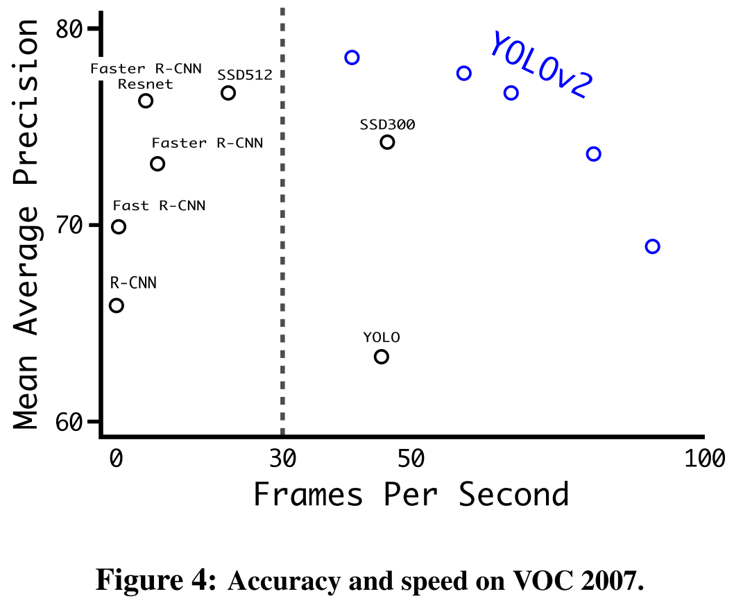
Performance

Improvements

• Add batch normalization
• Use high resolution classifier
• Convolve with anchor boxes
• Use k-means cluster for better prior bounding-boxes
• Use fine-grained features (pass through larger feature maps)
• Adopt multi-scale training
• Use Darknet-19 to be faster
• Use classification data to be stronger

Predicted variables

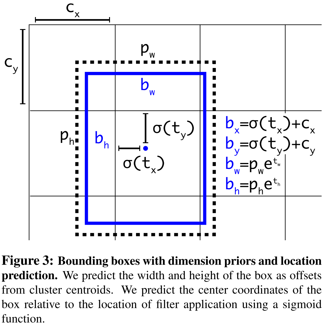
The network predicts 5 coordinates for each bounding box, $t_x,t_y,t_w,t_h$ and $t_o$. If the cell is offset from the top left corner of the image by $(c_x,c_y)$ and the bounding box prior has width and height $(p_w,p_h)$ then the predictions correspond to:

$$\begin{align} b_x=\sigma(t_x) + c_x, \ (1)\\ b_y =\sigma(t_y)+c_y, \ (2)\\ b_w=p_we^{t_w}, \ (3)\\ b_h=p_he^{t_h},\ (4)\\ Pr(object)*IOU(b, Object) = \sigma(t_o), \ (5) \end{align}$$

In original code, this part of calculation is:

#this paragraph is taken from 217~221 lines in models.py
#https://github.com/ultralytics/yolov3
#p-->(1,3,13,13,85), 13x13 grids, 81 classes (80+confidence) + 4 coordinate values
io = p.clone()  # inference output
io[..., :2] = torch.sigmoid(io[..., :2]) + self.grid  # xy - (1)(2)
io[..., 2:4] = torch.exp(io[..., 2:4]) * self.anchor_wh  # wh yolo method - (3)(4)
io[..., :4] *= self.stride
torch.sigmoid_(io[..., 4:]) # (5)

This is similar to the parameterization used by Fast R-CNN and Faster R-CNN.

Joint classification and detection

When our network sees a detection image we backpropagate loss as normal. For classification loss, we only backpropagate loss at or above the corresponding level of the label.

...When it sees a classification image we only backpropagate classification loss....

YOLOv3 - tech report 2018

Website: https://pjreddie.com/yolo/

Code: https://github.com/ultralytics/yolov3

Good illustration: 【论文解读】Yolo三部曲解读——Yolov3

Some "incremental" improvements on YOLOv2

J. Redmon and A. Farhadi. Yolov3: An incremental improvement. arXiv, 2018. 4

Performance

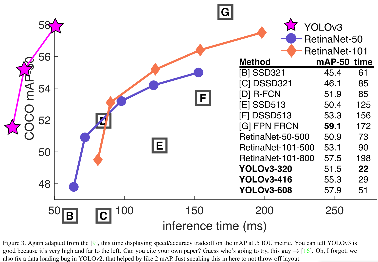
Structure

Source: https://zhuanlan.zhihu.com/p/76802514

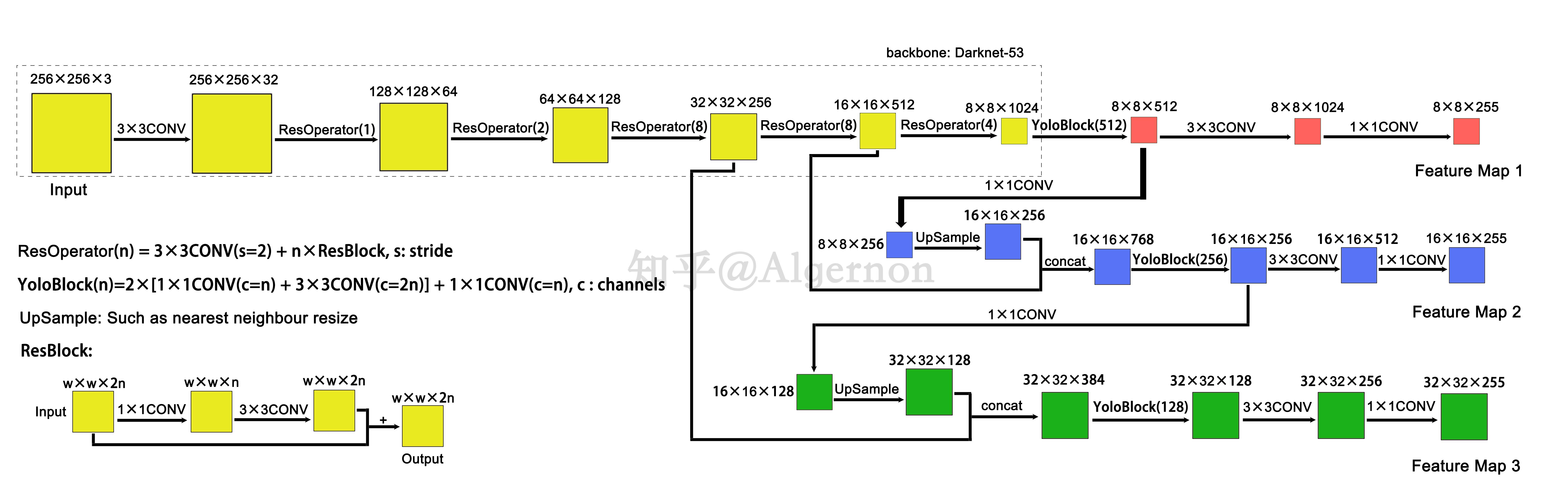
Adopt the idea of short-cut from ResNet, the idea of concatenate-multi-layer from DenseNet.

Changes:

• Adopt a new deeper backbone network : Darknet-53
• Deprecate the softmax layer for class prediction

Loss

The loss is still the combination of loss for location, size, confidence and class. But there are few changes.

Loss for location and size:

xxxxxxxxxx
# GIoU
pxy = ps[:, :2].sigmoid()
pwh = ps[:, 2:4].exp().clamp(max=1E3) * anchors[i]
pbox = torch.cat((pxy, pwh), 1)  # predicted box
giou = bbox_iou(pbox.t(), tbox[i], x1y1x2y2=False, GIoU=True)  # giou(prediction, target)
lbox += (1.0 - giou).sum() if red == 'sum' else (1.0 - giou).mean()  # giou loss

In mathematical form:

$A_c$ is the area of convex (smallest enclosing box).

Loss for confidence:

xxxxxxxxxx
BCEobj = nn.BCEWithLogitsLoss(pos_weight=ft([h['obj_pw']]), reduction=red)
#...
# Obj
tobj[b, a, gj, gi] = (1.0 - model.gr) + model.gr * giou.detach().clamp(0).type(tobj.dtype)  # giou ratio
#....
lobj += BCEobj(pi[..., 4], tobj)  # obj loss

In mathematical form:

Loss for classes:

xxxxxxxxxx
BCEcls = nn.BCEWithLogitsLoss(pos_weight=ft([h['cls_pw']]), reduction=red)
#...
# Class
if model.nc > 1:  # cls loss (only if multiple classes)
    t = torch.full_like(ps[:, 5:], cn)  # targets
    t[range(nb), tcls[i]] = cp
    lcls += BCEcls(ps[:, 5:], t)  # BCE

In mathematical form:

The final loass is a weighted sum of these three losses:

xxxxxxxxxx
#h is a dictionary of hyper-parameters
lbox *= h['giou']
lobj *= h['obj']
lcls *= h['cls']
#...
loss = lbox + lobj + lcls

SSD - ECCV 2016

Liu, Wei & Anguelov, Dragomir & Erhan, Dumitru & Szegedy, Christian & Reed, Scott. (2015). SSD: Single Shot MultiBox Detector. ECCV 2016

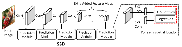
Strategy

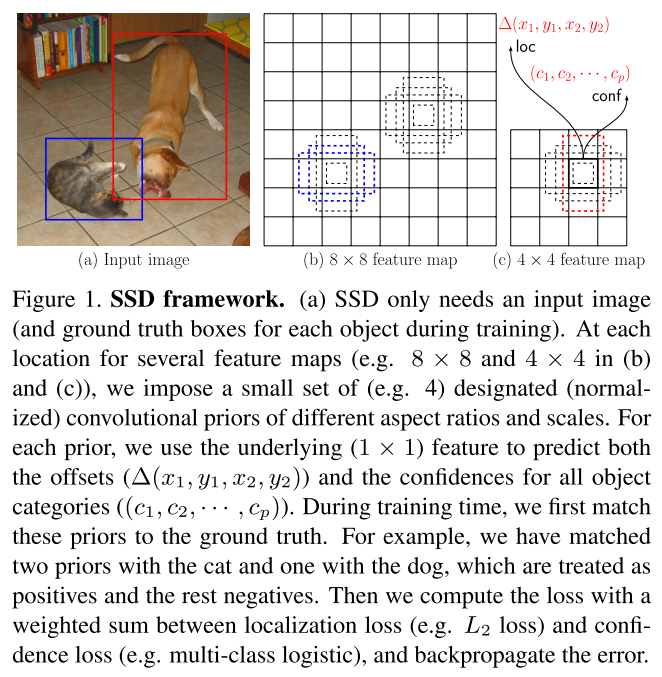
The overall process is just like YOLOv1, using a single network to predict class and location, but with differences as follow:

• Extract multiple feature maps from different spatial resolution (feature maps from multiple layers in backbone)
• Designate a series of prior bounding boxes of different aspect ratios and scales for each pixel

Structure

Xiongwei Wu, Doyen Sahoo, Steven C.H. Hoi. Recent Advances in Deep Learning for Object Detection. 2019. arXiv:1908.03673

Loss

The final loss consists of a confidence loss and a localization loss:

For the $i$ th prior, $c_i^p$ is the confidence for category $p$, $l_i$ is the $i$ th predicted box coordinates and $g_j^p$ is the $j$ th ground truth box coordinates of category $p$.

Match strategy:

• bipartite matching - ground truth box is greedily matched to the source box with best jaccard overlap (IoU)
• per-prediction matching - ground truth box is first matched using bipartite matching, and then use a jaccard overlap threshold to sift out several positive prior matches

RetinaNet - TPAMI 2017

Lin T Y , Goyal P , Girshick R , et al. Focal Loss for Dense Object Detection[J]. IEEE Transactions on Pattern Analysis & Machine Intelligence, 2017, PP(99):2999-3007.

It majorly focuses on the imbalance of positive and negative examples in object detection, especially in one-stage methods and a new loss function, focal loss, is proposed to cope with it.

Focal Loss

Instead, we propose to reshape the loss function to down-weight easy examples and thus focus training on hard negatives.

In which, $y\in{\pm1}$ specifies the ground-truth class and $p\in{[0,1]}$ is the model's estimated probability for the class with label $y=1$.

(1) When an example is misclassified and $p_t$ is small, the modulating factor is near 1 and the loss is uneffected. As $p_t \rightarrow 1$, the factor goses to $0$ and the loss for well-classified examples is down-weighted.

(2) The focusing parameter $\gamma$ smoothly adjusts the rate at which easy examples are down-weighted.

Vriants of focal loss involving sigmoid:

An example is correctly classified when $x_t>0$, in which case $p_t>0.5$.

Structure

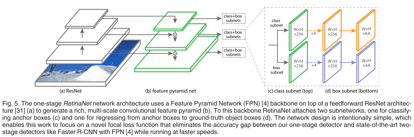
A classifier subnet and a regressor subnet are drawn out of feature maps of different scales (deeper feature maps are combined to current feature maps before processed by subnets). Focal loss is adopted for classifier subnet.

Anchor-free

The so called "anchor-free" should be more carefully rephrased as "anchor-prior-free". Although there is no explicit anchors in these methods, they implicitly use densely distributed anchors of fixed size.

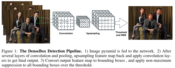
DenseBox - CVPR 2015

Code: https://github.com/CaptainEven/DenseBox

Huang L , Yang Y , Deng Y , et al. DenseBox: Unifying Landmark Localization with End to End Object Detection. CVPR, 2015.

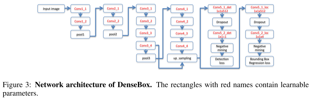
Structure

FCOS - ICCV 2019

Code: https://github.com/tianzhi0549/FCOS/

No anchor, but still with NMS as post processing.

Tian Z , Shen C , Chen H , et al. FCOS: Fully Convolutional One-Stage Object Detection. ICCV 2019.

Structure

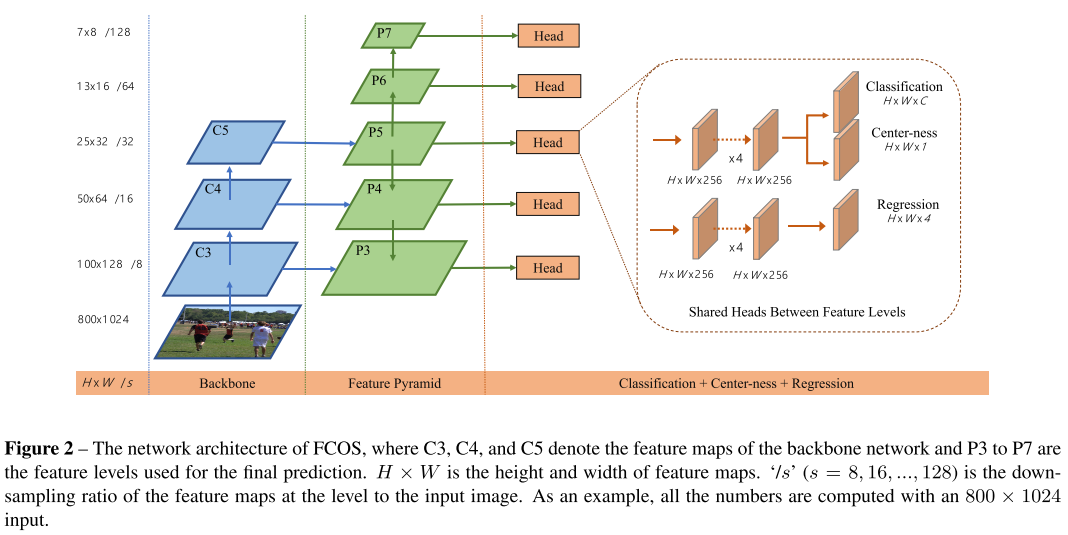
It's just like the structure of RetinaNet , but with different heads.

Loss

The final loss is a combination of classification loss and regression loss:

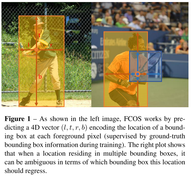
For each location $(x,y)$, a class probability vector $\bold{p}_{x,y}$ and a bounding-box reparameterized vector $\bold{t}_{x,y}$ is predicted. If a location $(x,y)$ is associated to a bounding box $B_i=(x_0^{(i)},y_0^{(i)},x_1^{(i)},y_1^{(i)},c^{(i)})\in{\mathbb{R^4}\times\{1,2,...,C\}}$, the regression target $\bold{t}^*=(l^*,t^*,r^*,b^*)$ is formulated as:

$L_{cls}$ is focal loss and $L_{reg}$ is the IoU loss. $N_{pos}$ denotes the number of positive samples. The summation is calculated over all locations on the feature maps $F_i\in\mathbb{R}^{H\times W\times C}$ .

More specifically, we firstly compute the regression targets $l^*,t^*,r^*$ and $b^*$ for each location on all feature levels. Next, if a location satisfies $max(l^*,t^*,r^*,b^*)$ > $m_i$ or $max(l^*,t^*,r^*,b^*)$ < $m_{i-1}$, it is set as a negative sample and is thus not required to regress a bounding box anymore. Here $m_i$ is the maximum distance that feature level $i$ needs to regress. In this work, $m_2, m_3, m_4, m_5, m_6$ and $m_7$ are set as 0, 64, 128, 256, 512 and $\infin$, respectively.

The center-ness target is calculated as (using BCELoss while training):

The NMS process is used to filter out bounding boxes with low center-ness for better performance.

CenterNet - 2019

Code: https://github.com/xingyizhou/CenterNet

This net could be view as a successor of CornerNet:

Law H , Deng J . CornerNet: Detecting Objects as Paired Keypoints. International Journal of Computer Vision, 2018.

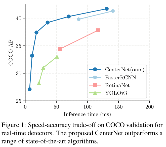
No anchor, no NMS. It's said that this paper was rejected by ECCV 2020 (why?)

X. Zhou, D. Wang, P. Krahenbuhl, Objects as points, in: arXiv preprint arXiv:1904.07850, 2019.

Performance

Objects as Points

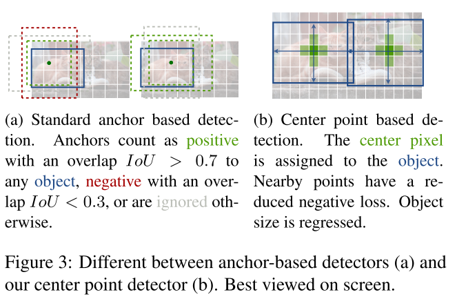
It represents a bounding-box by its center point and size and use a keypoint heatmap to estimate the center point and then regresses for the size of bounding-box.

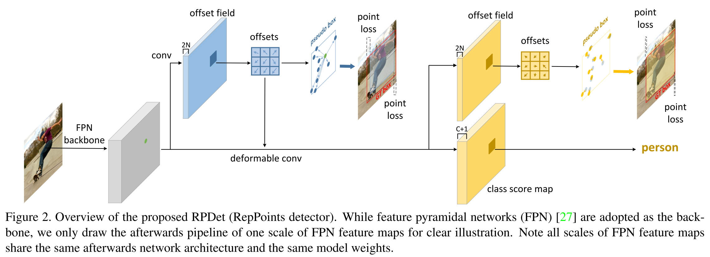
Structure

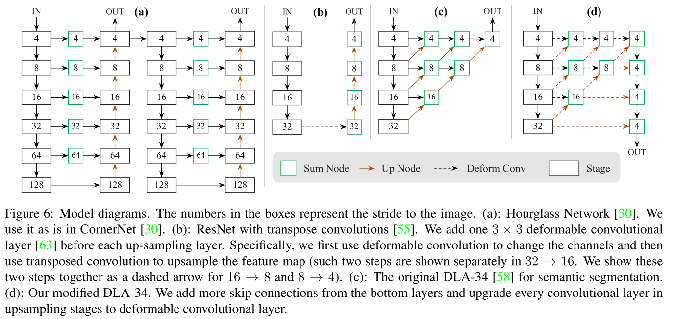
The overall structure is just like an auto-encoder, but the reconstructed image is a purposed heatmap rather than input itself.

Loss

The final loss consists of a keypoint loss, a size loss and an offset loss:

The keypoint loss is a type of focal loss:

A keypoint heatmap $\hat{Y}\in{[0,1]^{\frac{W}{R}\times\frac{H}{R}\times C}}$ is produced according to an input image $I\in{R^{W\times H\times 3}}$ with output stride $R$ and $C$ keypoint typs (object categories). $\hat{Y}_{x,y,c}=1$ if a keypoint of type $c$ is detected in $(x,y)$, else $\hat{Y}_{x,y,c}=0$ , which is the background.

For each ground truth keypoint $p\in{R^2}$ of class $c$, a low-resolution equivalent is computed as $\tilde{p}=[\frac{p}{R}]$. All ground truth keypoints are then splat onto a heatmap $Y\in{[0,1]^{\frac{W}{R}\times\frac{H}{R}\times C}}$ using a Gaussian kernel $Y_{xyc}=exp(-\frac{(x-\tilde{p}_x)^2+(y-\tilde{p}_y)^2}{2\sigma_p^2})$, in which $\sigma_p$ is an object size-adaptive standard deviation.

In short, a dotted heatmap of ground-truth center points is blurred with an adaptive Gaussian kernel.

The offset loss is as:

An additional local offset $\hat{O}\in{R^{\frac{W}{R}\times\frac{H}{R}\times 2}}$ is predicted to recover the discretization error caused by the output stride $R$ for each center point $p$.

The size loss is as:

In which, $s_k=(x_2^{(k)}-x_1^{(k)},y_2^{(k)}-y_1^{(k)})$ is the ground-truth size of object $k$ with a bounding-box of $(x_1^{(k)},y_1^{(k)},x_2^{(k)},y_2^{(k)})$ , $\hat{S}\in{R^{\frac{W}{R}\times\frac{H}{R}\times 2}}$ is the predicted size for all object categories.

In short, for each pixel point on the down-sampled map of $\frac{W}{R}\times\frac{H}{R}$, a size of $2$ dimensions is predicted.

Inference

1. For each category, extract top 100 peaks (value greater or equal to its 8-connected neighbors) of heatmap.
2. For center point prediction $(\hat{x}_i,\hat{y}_i)$, with size prediction $(\hat{w}_i,\hat{h}_i) = \hat{S}_{\hat{x}_i,\hat{y}_i}$ and offset prediction $(\delta\hat{x}_i,\delta\hat{y}_i)=\hat{O}_{\hat{x}_i,\hat{y}_i}$, a bounding-box is produced at location $(\hat{x}_i+\delta\hat{x}_i-\hat{w}_i/2,\hat{y}_i+\delta\hat{y}_i-\hat{h}_i/2,\hat{x}_i+\delta\hat{x}_i+\hat{w}_i/2,\hat{y}_i+\delta\hat{y}_i+\hat{h}_i/2)$ .

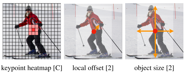
RPDet- 2019

Ze Yang, Shaohui Liu, Han Hu, Liwei Wang, Stephen Lin. RepPoints: Point Set Representation for Object Detection. arXiv:1904.11490

The major idea of this paper is to replace bounding-box with reppoints, a set of keypoints to represent the location of an object.

The bounding box representation considers only the rectangular spatial scope of an object, and does not account for shape and pose and the positions of semantically important local areas, which could be used toward finer localization and better object feature extraction.

RepPoints representation

A set of $n$ adaptive sample points is used to locate an object:

The refinement of RepPoints is expressed as:

In which, $\{(\Delta x_k,\Delta y_k)\}_{k=1}^n$ are the predicted offsets.

A pre-defined converting function $\mathcal{T}:\mathcal{R}_P\rightarrow\mathcal{B}_P$ is used to convert RepPoints into a pseudo box.

Loss

The learning of RepPoints is driven by both an object localization loss and an object recognition loss.

The object localization loss is computed using smooth L₁ distance between the pseudo box converted from RepPoints and the ground-truth bounding box.

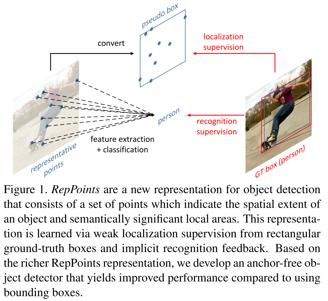
Structure

The overall process is similar to a two-stage method:

1. A coarse set of offsets from a center point is first learned and used to generate a coarse set of RepPoints.
2. The object localization loss is then used to refine the RepPoints.

In inference, NMS (σ = 0.5) is employed to postprocess the results, following RetinaNet. (?)

Performance

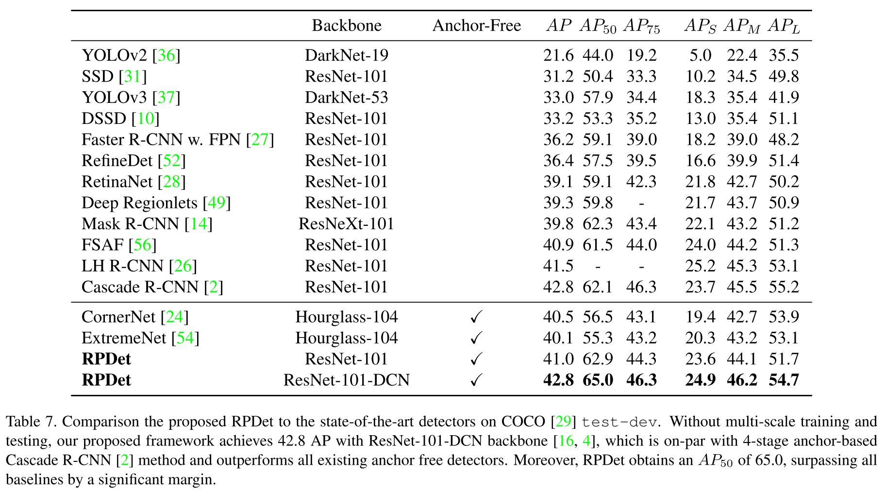
Frontier

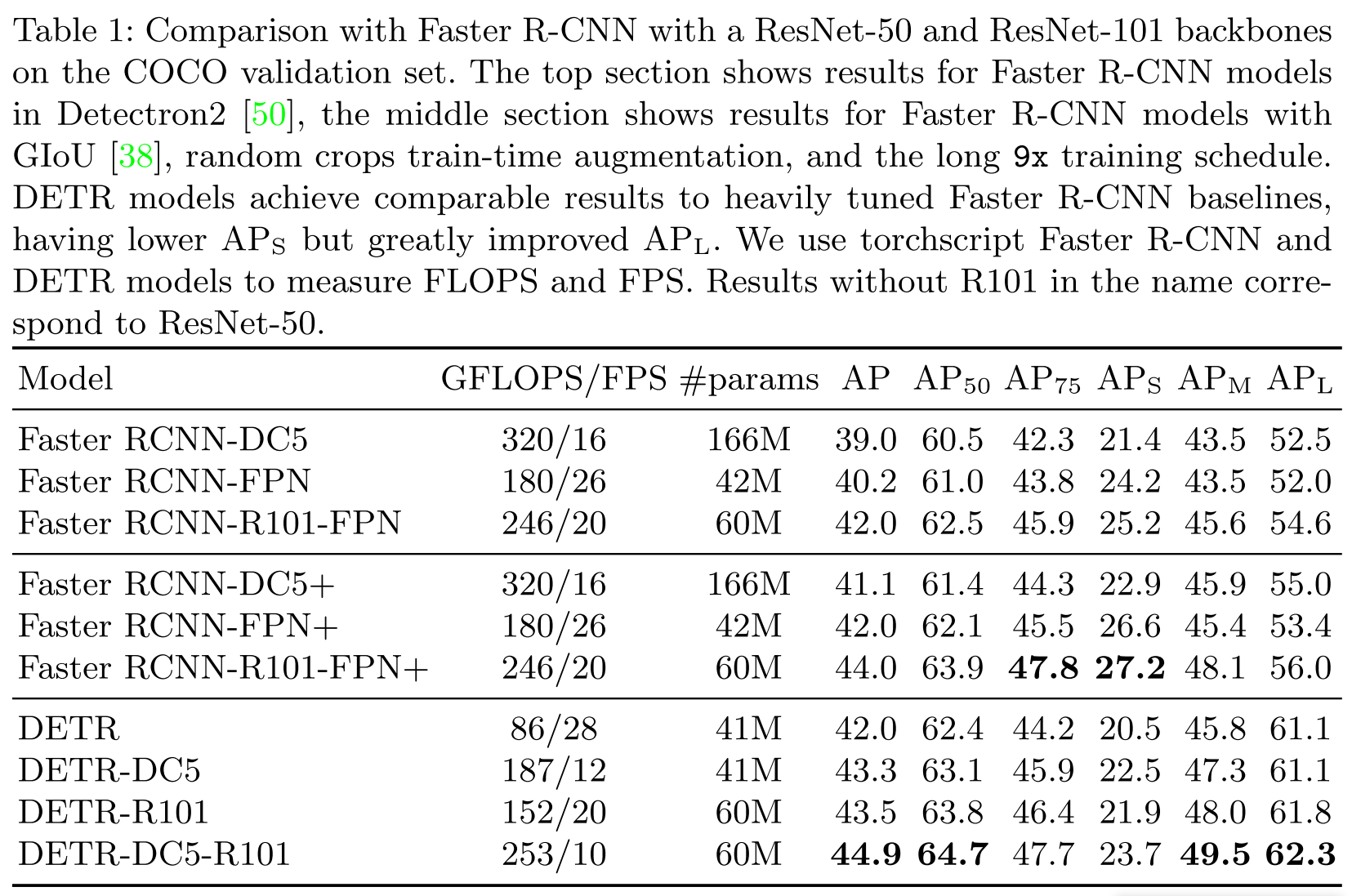
DETR - ECCV 2020

Code: https://github.com/facebookresearch/detr

Nicolas Carion, Francisco Massa, Gabriel Synnaeve, Nicolas Usunier, Alexander Kirillov, and Sergey Zagoruyko. End-to-End Object Detection with Transformers. arXiv:2005.12872

This paper migrates the idea from NLP to the problem of object detection, which may be a game changer.

Structure

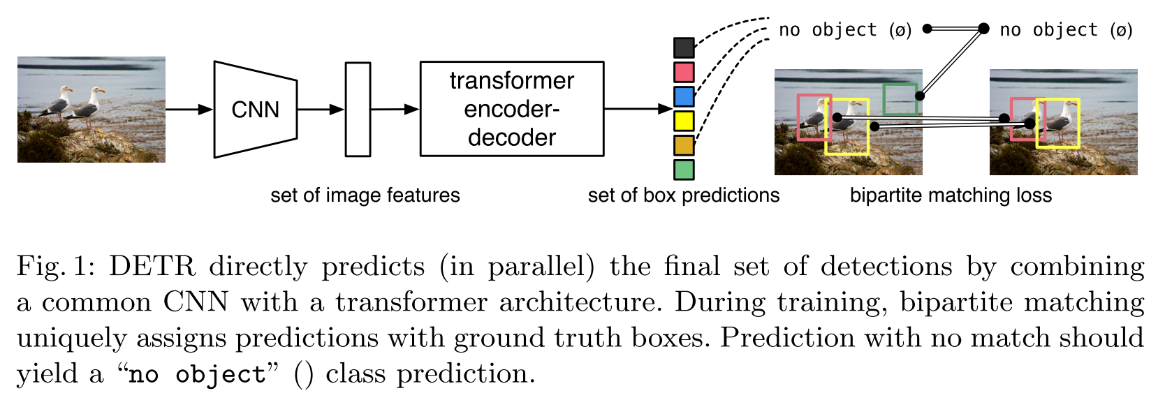
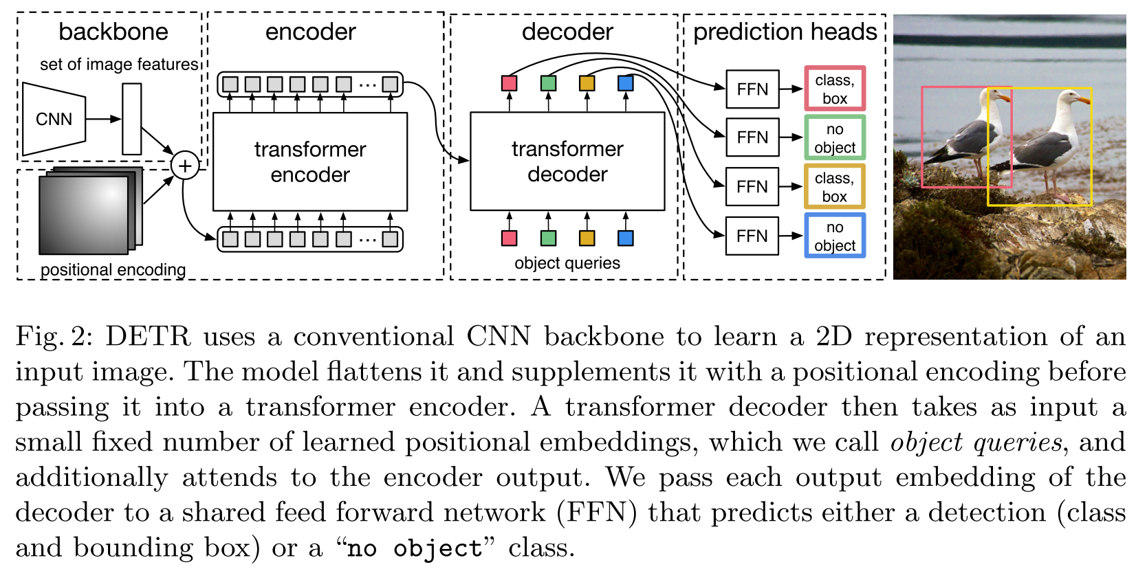
The strategy is very freshing:

1. Use CNN to extract features from the input image.
2. View the extracted features as a sequence and put it into a translator network (built with transformers).
3. Obtain the detected objects from the output sequence translated from the input.

Loss

For a ground-truth set of objects $y$ (a set of size $N$ padded with $\empty$) and $N$ predicted sets $\hat{y}=\{\hat{y}_i\}_{i=1}^N$, a bipartite matching between these two sets is found with the search of a permutation of $N$ elements $\sigma\in{\mathcal{S}_N}$(using Hungarian algorithm (How?)):

In which, $y_i=(c_i,b_i)$ denotes the target class label $c_i$ and the ground-truth bounding box $b_i\in{[0,1]^4}$; $\hat{p}_{\sigma(i)}(c_i)$ is the predicted probability of index $\sigma(i)$ to be class $c_i$; $\hat{b}_{\sigma(i)}$ is the predicted box for index $i$ .

The final loss is a combination of an object set prediction loss and a bounding box loss:

In which, $\hat{\sigma}$ is the optimal assignment computed before. And the bounding box loss is defined as:

The $\mathcal{L}_{iou}$ here is the generalized intersection over union (GIoU) loss. Same as that in YOLOv3.

In short, for each predicted set, a optimally matched permutation is found using Hungarian algorithm, for the optimal permutation of predicted set, the loss is designed to minimize the corresponding bounding box error and maximize the predicted probability for the correct class for each objects in it.

Auxiliary decoding losses. We found helpful to use auxiliary losses [1] in decoder during training, especially to help the model output the correct number of objects of each class. We add prediction FFNs (Feed-Forward Networks) and Hungarian loss after each decoder layer. All predictions FFNs share their parameters. We use an additional shared layer-norm to normalize the input to the prediction FFNs from different decoder layers.

Performance