Summarized Survey of Few-shot Learning

By LI Haoyang 2020.10.12 ~ 2020.10.13

This note is summarized from a review, therefore, no quote is specified, most of the following sentences are directly taken from the original article.

Content

Few-shot learning: a survey

YAQING WANG, QUANMING YAO. Few-shot Learning: A Survey. 2019. arXiv:1904.05046

Few-short learning aims to improve the model's ability to generalize over training on a small dataset. FSL can learn new task of limited supervised information by incorporating prior knowledge.

Problem definition

Start from the definition of machine learning, which is:

A computer program is said to learn from experience $E$ with respect to some classes of task $T$ and performance measure $P$ if its performance can improve with $E$ on $T$ measured by $P$. (Machine learning by Mitchell)

FSL is a special case of machine learning, which exactly targets at getting good learning performance with limited supervised information:

Few-Shot Learning (FSL) is a type of machine learning problems (specified by $E$, $T$ and $P$) where $E$ contains little supervised information for the target $T$.

The scenarios of FSL can be summarized as:

• Test bed for human-like learning.
• Few-shot to reduce data gathering effort and computation cost.
• Few-shot due to rare cases. (some tasks are naturally few-shot)

Therefore, FSL methods combine prior knowledge with available supervised information in E to make the learning of the target T feasible

Relevant problems

• Semi-supervised learning

  It learns the optimal hypothesis $o^*$ from input $x$ to output $y$ by experience $E$ consisting of both labeled and unlabeled examples.

  • Positive-unlabeled learning - only positive and unlabeled samples are given
  • Active learning - select informative unlabeled data to query an oracle for output $y$

• Imbalanced learning

  It learns from experience $E$ with severely skewed distribution for output $y$.

• Transfer learning

  It transfers knowledge learned from source domain and source task where sufficient training data is available, to target domain and target task where training data is limited.

  • Domain adaptation - where the tasks are the same but the domain is different.
  • Zero-shot learning - recognize new class with no supervised training examples by linking them to existing classes that one has already learned. (Cluster?)

• Meta-learning

  It improves performance $P$ on task $T$ by data set of the task $T$ and the meta knowledge extracted across tasks by a meta-learner.

  

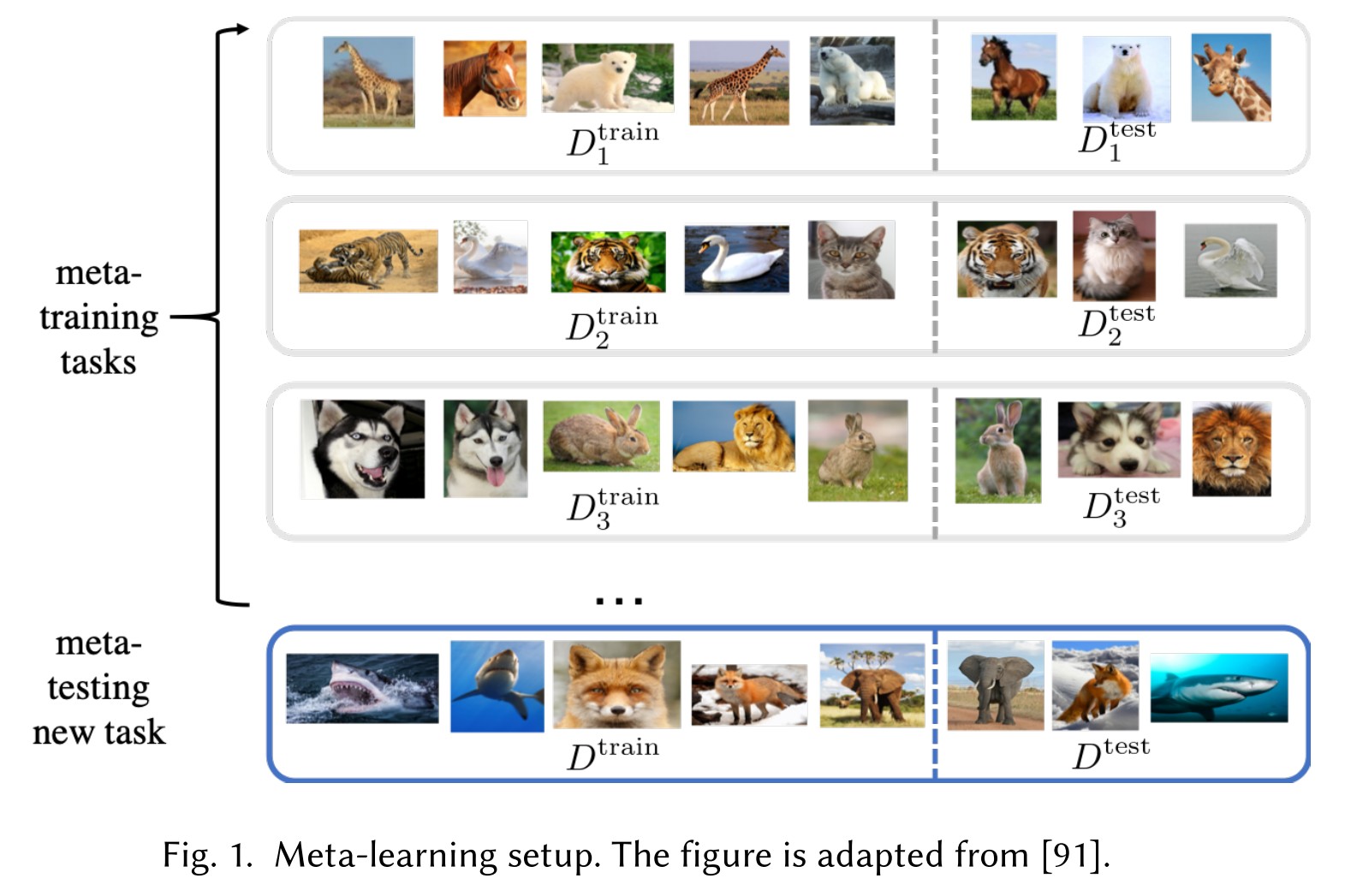
  Let $p(T)$ be the distribution of task $T$. In meta-learning, it learns from as set of tasks $T_s\sim p(T)$. Each task $T_s$ operates on data set $D_{T_s}$ of $N$ classes where $D_{T_s}=\{D_{T_s}^{train},D_{T_s}^{test}\}$ with $D_{T_s}^{train}=\{(x_{T_s}^{(i)},y_{T_s}^{(i)})\}$ and $D_{T_s}^{test}=\{(x_{T_s}^{test},y_{T_s}^{test})\}$. Each learner learns from $D_{T_s}^{train}$ and measures test error on $D_{T_s}^{test}$. The parameter $\theta$ of meta-learner learns to minimize the error across all learners by:

  $$\theta=\arg\min_{\theta}\Bbb{E}_{T_s\sim p(T)}l_{\theta}(D_{T_s})$$

  In meta-testing, another disjoint set of tasks $T_t\sim p(T)$ is used to test the generalization ability of meta-learner. Each $T_t$ works on data set $D_{T_t}$ of $N^{'}$ classes where $D_{T_t}=\{D_{T_t}^{train},D_{T_t}^{test}\}$ with $D_{T_t}^{train}=\{(x_{T_t}^{(i)},y_{T_t}^{(i)})\}$ and $D_{T_t}^{test}=\{x_{T_t}^{test}\}$. Finally the learner learns from $D_{T_t}^{train}$ and tests on $D_{T_t}^{test}$ to obtain the meta-learning testing error.

  It appears to me that meta-learning is an ensemble of classifiers trained on partial dataset.

Core issue of FSL

Start from machine learning problem, improving with $E$ on $T$ measured by $P$, formulated as:

In this form, learning is about algorithm searching in $\cal{H}$ for the $\theta$ which parameterizes the hypothesis $h\in\cal{H}$ chosen by model that best fit data $D^{train}$.

Decomposition of error

Let $\hat{y}$ be the prediction of some function $o$ for $x$. To solve the problem defined above, the essence is to minimize the expected risk $R$ (i.e. losses measured with respect to $p(x,y)$), formulated as:

Since $p(x,y)$ is unknown in practice, the empirical risk $R_I(h)$ is used to estimate the expected risk $R_I(h)$, defined as the average of the sample loss over the training data set:

The learning is done by empirical risk minimization.

In short, empirical risk minimization assumes that every sample in the training set is of the same probability.

Let:

• $o^*=\arg\min_f R(o)$, the real but unreachable solution
• $h^*=\arg\min_{h\in \cal{H}}R(h)$, the unreachable best solution in $\cal{H}$
• $h_I^*=\arg\min_{h\in\cal{H}}R_I(h)$, the reachable best solution in $\cal{H}$

The total error of learning taken with respect to the random choice of training set can be decomposed into:

• Approximation error $\cal{E}_{app}(H)$ measures how closely functions in $\cal{H}$ can approximate the optimal solution $o^*$.
• Estimation error/Generalization error $\mathcal{E}_{est}(\mathcal{H},I)$ measures the effect of minimizing the empirical risk $R_I(h)$ rather than the expected risk $R(h)$.

Given the analysis above, learning to reduce the total error can be attempted from the perspective of data which offers $D^{train}$, model which offers $\cal{H}$ and algorithm which searches through $\cal{H}$ for the parameter $\theta$ of the best $h$.

Sample complexity

For $0<\epsilon, \delta<0.5$, sample complexity $S$ is an integer such that for $I\ge S$, we have:

In short, sample complexity is the number of samples we need for the estimation error to be small enough.

For infinite space $\cal{H}$, its complexity can be measured in terms of VapnikâĂŞChervonenkis(VC) dimension, defined as the size of the largest set of inputs that can be shattered (split in all possible ways) by $\cal{H}$. The sample complexity $S$ is tightly bounded as:

The sample complexity increases with more complicated $\cal{H}$, higher probability $(1-\delta)$ that the learned $h_I$ is approximately correct and higher demand of optimization accuracy of algorithm.

Unreliable empirical risk minimizer

For estimation error, we have:

which means more examples can help reduce estimation error. Besides, there is (why?):

Thus in common setting of supervised learning task, empirical risk minimizer $h_I$ can provide a good and stable approximation $R(h_I)$ to the best possible $R(h^*)$ for $h$ in $\cal{H}$.

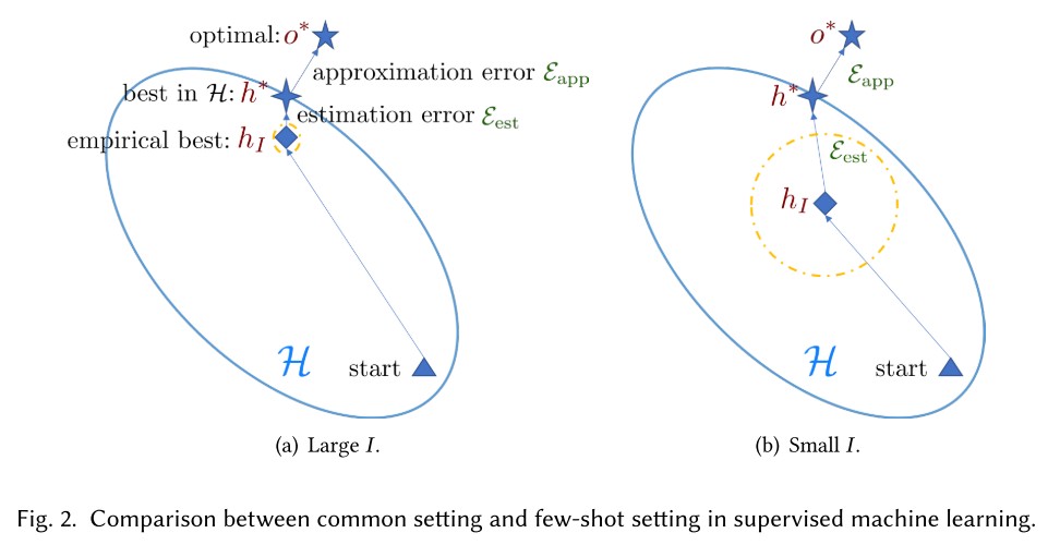
However, in the setting of few-shot learning where the number of available examples $I$ is smaller than the required sample complexity $S$. The empirical minimizer $h_I$ is no longer reliable, which is the core issue in FSL.

Taxonomy of current works

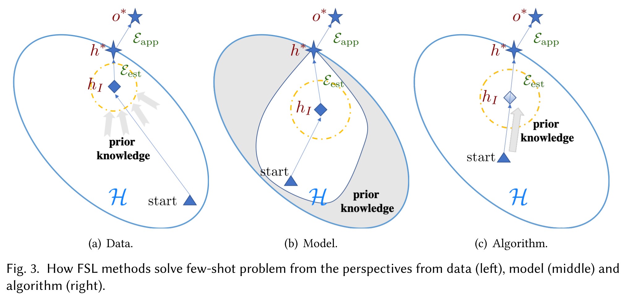
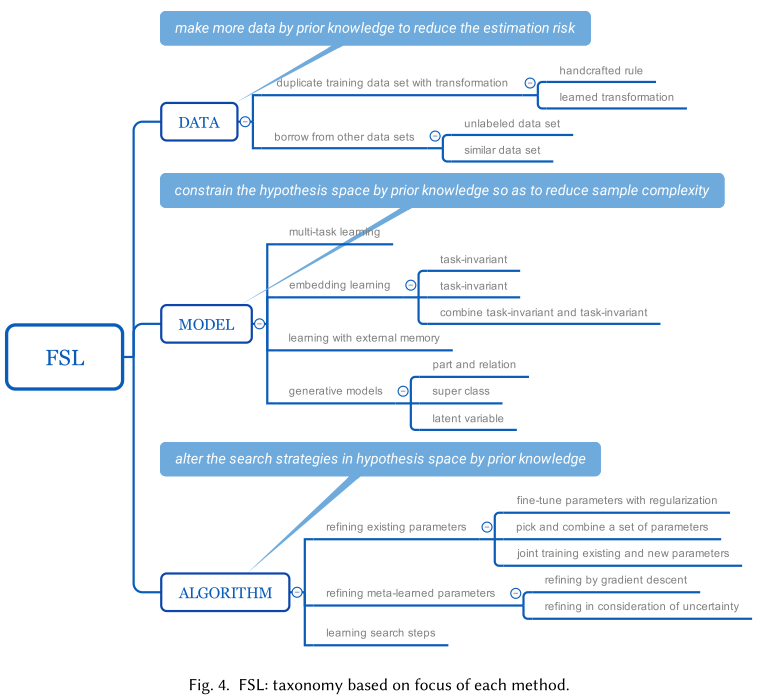
The existing works deal with the problem of unreliable empirical risk minimizer via the following perspectives:

• Data

  Use prior knowledge to augment $D^{train}$.

• Model

  Design $\cal{H}$ based on prior knowledge in experience $E$ to constrain the complexity of $\cal{H}$ and reduce its sample complexity $S$.

• Algorithm

  Use prior knowledge for better initial point or better search steps. (Meta-learning etc.)

Data focused approaches

Since few-shot suffers from the limited amount of data, the intuitive way to handle it is to augment training set $D^{train}$ with more data.

Duplicate training data with transformations

This stratgey augments $D^{train}$ by duplicating each $(x^{(i)},y^{(i)})$ into several samples with some transformation to bring in variation. These transformations are as follows:

• Handcrafted Rule

  Translating, flipping, shearing, scaling, reflecting, cropping and rotating,etc.

• Learned Transformation

  This strategy uses the prior learned transformation to augment $D^{train}$.

Direct use of handcrafted rule in FSL without considering the task or desired data property available in $D^{train}$ can make the estimation of distribution easily go stray. Hence it can only mediate rather than solve FSL problem and is only used as a pre-processing step for image data.

Using learned transformations can augment more suitable samples as it is data-driven and exploit prior knowledge akin to $D^{train}$ or task $T$. However, this prior knowledge needed to be extracted from similar tasks, which may not always be available and can be costly to collect.

Borrow from other data sets

This strategy borrows samples from other data sets and adapts them to be like sample of the target output, so as to be augmented to the supervised information $D^{train}$.

• Unlabeled Data Set

  This strategy uses a large set of unlabeled samples $D^{unlabeled}$ as prior knowledge, which possibly contains samples of the same label as $y^{(i)}$.

  The crux is to find the samples with the same label and add them to augment $D^{train}$.

• Similar Data Set

  This strategy augments $D^{train}$ by aggregating samples pairs from other similar (in classes) data sets with many-shot.

  The underlying assumption is that the underlying hypothesis $o^*$ applies to all classes, and the similarity between $x$ of classes can be transferred to $y$ of classes. Therefore, new samples can be generated as a weighted average of sample pairs of classes of the similar data set, where the weight is usually some similarity measure.

The use of $D^{unlabeled}$ is cheap but of lower quality.

Similar data set is more informative, but the collecting of it may be laborious and determining the key property of similarity can be objective.

Due to the imprecise prior knowledge guiding the augmentation (lack of $p(x,y)$), the generation of new samples is not precise. The gap between the estimated one and the ground truth largely interferes the data quality, even leading to concept drift.

Model focused approaches

Another approach is to constrain the hypothesis space $\cal{H}$ determined by the model as a parameterized hypothesis $h(\cdot;\theta)$.

Multitask learning

This strategy learns multiple learning tasks spontaneously, exploit the generic information shared across tasks and specific information of each task. These tasks are usually related.

When the tasks are from different domains, it's also called domain adaptation.

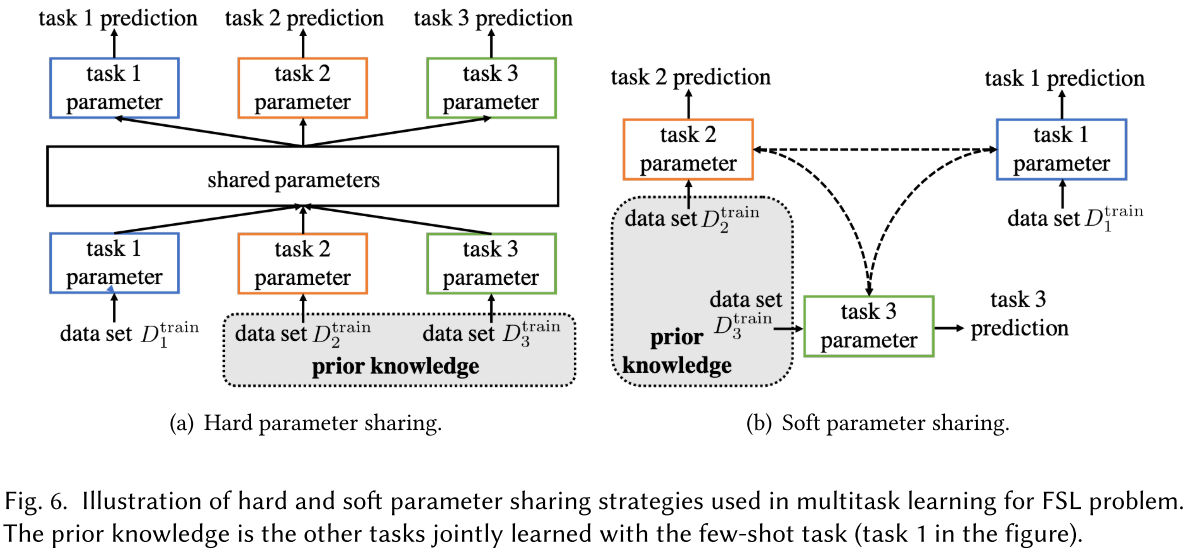
As these tasks are related, they are assumed to ve similar or overlapping hypothesis space $\mathcal{H}_{T_t}$, this is done explicitly by sharing parameters among these tasks, which can be viewed as a way to constrain each $\mathcal{H}_{T_t}$ by other jointly learned tasks.

• Hard Parameter Sharing

  It explicitly shares parameter among tasks to promote overlapping $\mathcal{H}_{T_t}$ and additionally learns a task-specific parameter for each task.

  It's actually the prevailing methodology in object detection, where the regression head shares the same parameters in deep layers with the classification head.

• Soft Parameter Sharing

  It only encourages parameters of different tasks to be similar, resulting similar $\mathcal{H}_{T_t}$, while each of them still has its own hypothesis space $\mathcal{H}_{T_t}$ and parameter $\theta_{T_t}$. This can be done by regularizing $\theta_{T_t}$.

  If the relation between $T_t$ are given, this regularizer can become a graph Laplacian regularizer on the similarity graphs of $\theta_{T}$, then this relations can guide information flow between $T_t$.

Embedding learning

I think it's also named as metric learning.

This strategy learns a hypothesis space $\mathcal{H}$ which embeds $x^{(i)}\in\mathcal{X}\sube\Bbb{R}^d$ to a smaller embedding space $z^{(i)}\in\mathcal{Z}\sube \Bbb{R}^m$, where the similar and dissimilar pairs can be easily identified.

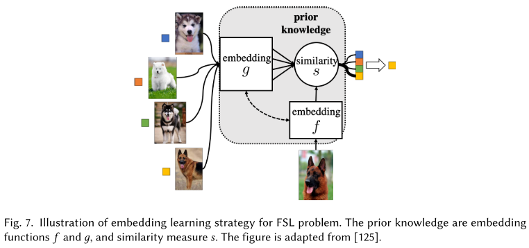
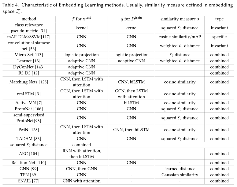
The embedding function is mainly learned by prior knowledge and can additionally uses $D^{train}$ to bring in task-specific information. The training sample $x^{(i)}\in D^{train}$ and the testing sample $x^{test}\in D^{test}$ are embedded differently by $g$ and $f$. The prediction is then done by assigning $x^{test}$ to the class of the most similar $x^{(i)}\in D^{train}\sube \mathcal{Z}$.

• Task-specific

  It learns an embedding function tailored to data distribution $D$. Given the few-shot in $D^{train}$, the sample complexity $S$ is largely reduced by enumerating all pairwise comparison between examples $D^{train}$ as input pairs. Then a model is learned to verify whether the input pairs have the same or different $y$.

• Task-invariant

  It learns embedding function from a large set of data sets $D_c, D\not\sub D_c$.The assumption is that if many data sets are well-separated on $\mathcal{Z}$ embedded by $\mathcal{H}$, it can be general enough to work well for $D$ without retraining.

• Combine Task-invariant and Task-specific

  It learns to adapt the generic task-invariant embedding space learned from prior knowledge by task-specific information contained in $D^{train}$.

This is also the prevailing use of pretrained CNN as feature extractor in literature.

Learning with external memory

This strategy memorizes the needed knowledge in an external memory to be retrieved or updated, hence relieves the burden of learning and allows fast generalization.

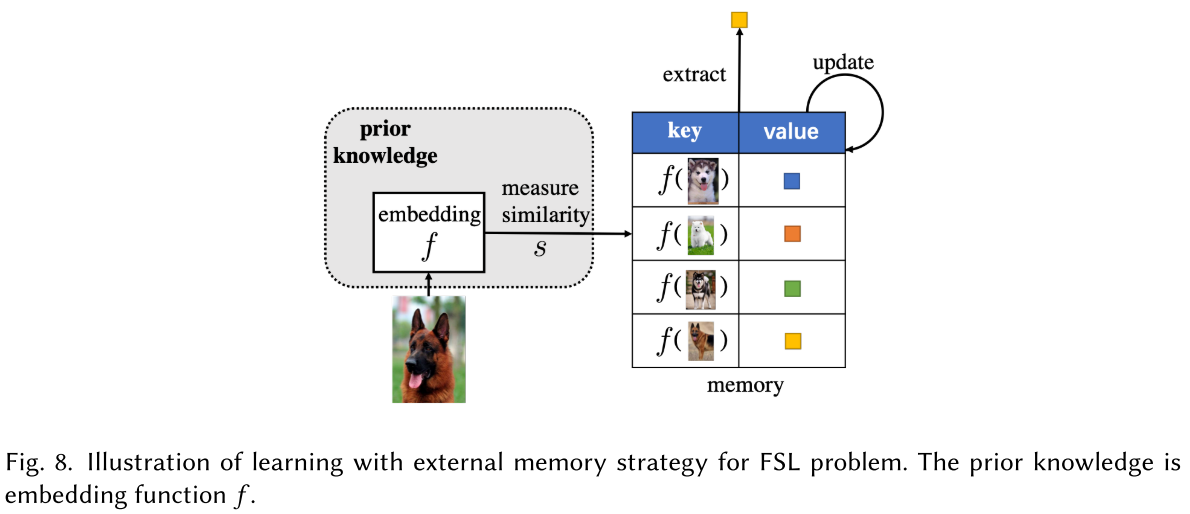
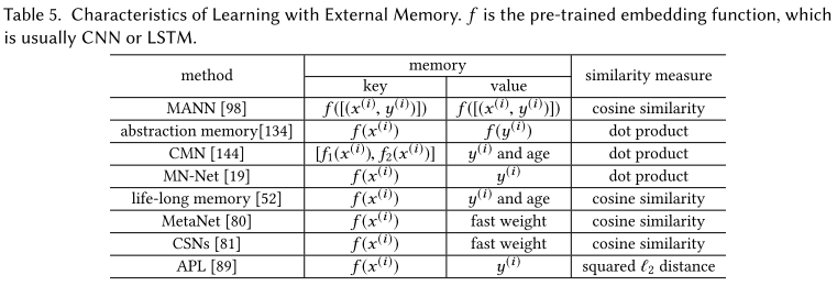
Denote memory as $M\in\Bbb{R}^{b\times m}$, which has $b$ memory slots $M(i)\in\Bbb{R}^m$. Given a sample $x^{(i)}$, it first embedded by $f$ as query $q\in\Bbb{R}^m$, then it attends to each $M(i)\in\Bbb{R}^k,i=1,\dots,b$ through some similarity measure $s$, e.g. cosine similarity, based on which the prediction is then given.

When a new sample comes, relevant contents are extracted from the memory and combined into the local approximation for this sample. The prediction is then made based on the updated approximation.

• Update the least recently used memory slot (e.g. MANN)
• Update by location-based addressing of neural Turing machine (e.g. neural Turing machine)
• Update according to age of memory slots (e.g. Life-long memory)
• Only update the memory when the loss is high
• Use the memory as storage only and wipe it out across tasks (e.g. MetaNet)
• Aggregate the new information into the most similar one (e.g. Memory Matching Networks)

It relies on human knowledge to design a desired rule. The existing works do not have a clear winner. How to design or choose update rules according to different setting automatically are important issues.

It sounds rather traditional to use memory solving the FSL problem.

Generative models

Here, the generative modeling methods refer to methods involve learning $p(x,y)$. It uses both prior knowledge and $D^{train}$ to obtain the estimated distribution.

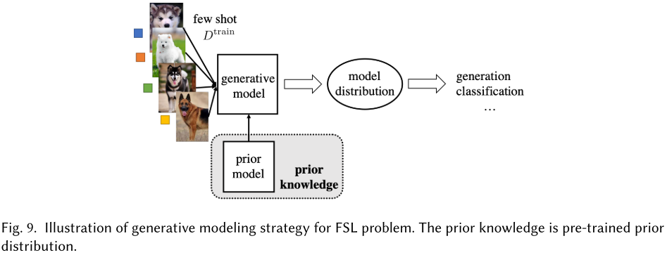
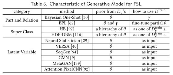
Prior probability distributions of each $h\in\mathcal{H}$ are learned from a set of $C$ data sets $D_c$, which is usually large and disjoint with $D^{train}$, it then updates the probability distribution over $D^{train}$ for prediction.

By Bayes' rule, we have:

In which, $\theta$ is the parameter of $h\in\mathcal{H}$. If $D^{train}$ is large enough, we can use it to learn a well-peaked $p(\theta|y,D^{train})$, and obtain $\theta$ using:

• Maximum Likelihood Estimation (MLE) $\theta^{ML}=\arg\max_{\theta}p(\theta|y,D^{train})$
• Maximum a posterior (MAP) $\theta^{MAP}=\arg\max_{\theta}p(\theta|y,D^{train})p(\theta)$

For FSL, generative models assume $\theta$ is transferable across different $y$ (e.g. classes). Hence $\theta$ can be instead learned from a large set of data sets $D_c$.

• Part and Relation (e.g. Bayesian One-Shot, BPL)

  This strategy learns part and relation (a.k.a. $\theta$) from a large set of $D_c$ as prior knowledge.

  For $(x^{(i)},y^{(i)})\in D^{train}$, the model needs to infer the correct combination of related parts and relations, then decides which target class this combination belongs to.

• Super Class (e.g. HB, HDP-DBM)

  This strategy clusters similar classes by unsupervised learning, it finds the best $\theta$ which parameterize $h\in\mathcal{H}$ for these super classes as prior knowledge.

  A new class is first assigned to super class, then finds the best $h$ through adapting the super class's $h$.

• Latent Variable

  This strategy models latent variables with no implicit meaning shared across classes.

All methods approaching from model design $\cal{H}$ based on prior knowledge in experience $E$ to constrain the complexity of $\cal{H}$ and reduce its sample complexity $S$.

• Multitask learning constrains $\cal{H}$ learned by $D^{train}$ regularized by a set of tasks jointly learned. When these tasks are highly related, they can guide each other in complement and prevent overfitting problem.
• Embedding learning methods learns to embed samples from $\cal{H}$ to a smaller embedding space, where the similar and dissimilar pairs can be easily identified.
• Learning with external memory refines and re-interprets each sample by $D^{train}$ stored in memory consequently reshaping $\cal{H}$.
• Generative model for FSL learns prior probability from prior knowledge, hence shaping the form of $\cal{H}$. It has good interpretability, causality and compositionality.

Algorithm focused approaches

The so-called algorithm here denotes the strategy to search for the parameter of the best $h$ in hypothesis space $\cal{H}$. The prevailing algorithms for this search root from the gradient descent method:

In which, $f_t(\theta)=l(h(x^{(t)};\theta),y^{(t)})$, measuring the loss incurred by $\theta$ in $t$-th iteration.

The unreliable empirical risk minimizer makes this approach unreliable. The algorithm-centered methods aim to improve the search process for the best $\theta$ by taking advantage of prior knowledge.

Refining existing parameters $\theta^0$

This strategy takes $\theta^0$ from a pre-trained model as a good illustration, and adapts it to $\theta$ by $D^{train}$.

It assumes that since $\theta^0$ captures general structures by learning from large-scale data, it can be adapted using a few iterations to work well on $D$.

• Fine-tune $\theta^0$ with regularization

  

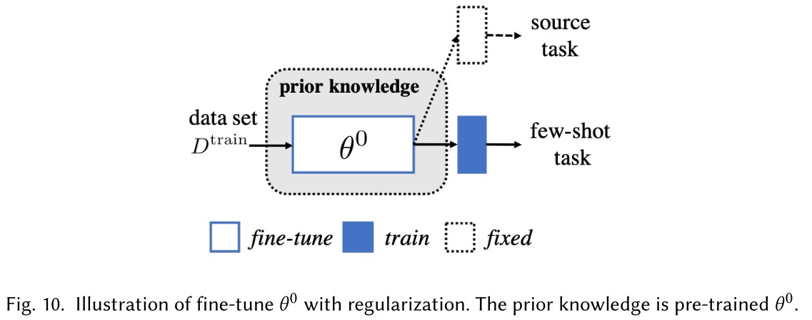
  It fine-tunes the pre-trained model to $D^{train}$ with regularization to prevent overfitting.

• Pick and combine a set of $\theta^0$

  

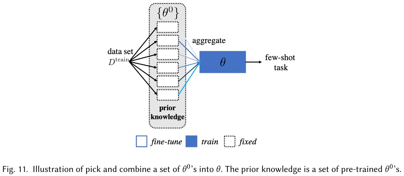
  It pick from a set of $\theta^0$ from models trained for relevant tasks and combine them into the suitable initialization to by adapted by $D^{train}$.

• Fine-tune $\theta^0$ with new parameters

  

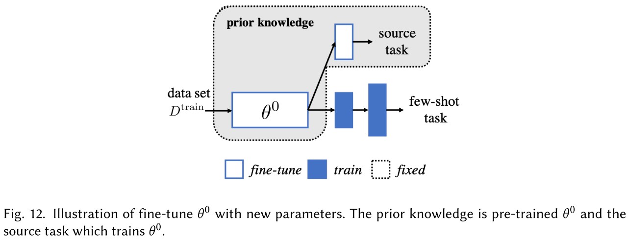
  It fine-tunes $\theta^0$ from the pre-trained model to $D^{train}$ with extra parameters $\delta$ attached.

Most of these designs are still heuristic, lack of certain interpretability.

Refining meta-learned $\theta$

This strategy directly targets at $h^*$.

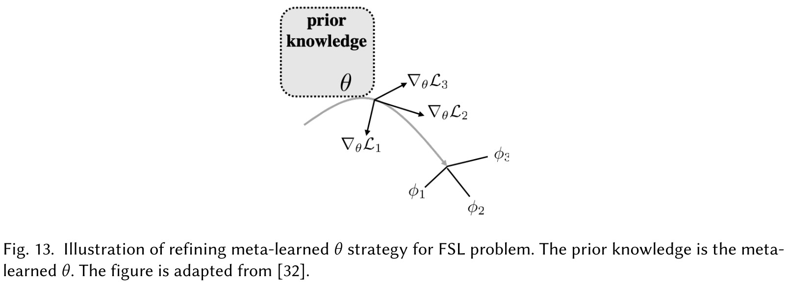
Iteratively, the meta-learner parameterized by $\theta$ provides information about parameter updates to parameter $\psi_T$ of task $T$'s learner and the learner returns error signals to meta-learner to improve it.

• Refining by gradient descent (e.g. MAML)

  It simply refines the meta-learned $\theta$ by gradient descent.

• Refining in consideration of uncertainty

  Basically, it models the distribution of $\theta$ and tries to pick a task-specific $\theta^0$ based on $\theta$.

For this approach to work, the tasks over which the meta-learner learns should be related intuitively.

Learning search steps

Its idea is to automatically produce the proper gradient update steps, a good step size, or even a good initialization to start with.

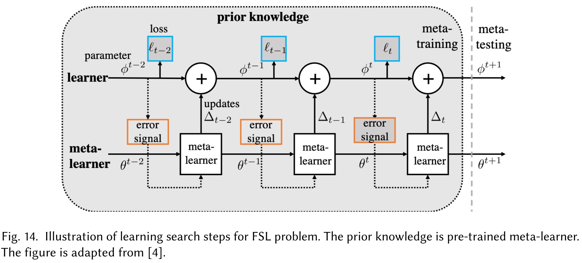
It appears to me as a cooperated training of a meta-learner and a target learner.

All methods focused on algorithm take advantage of prior knowledge to search for the $\theta$ which parameterizes the best $h\in \mathcal{H}$.

The former two both aim at a better initialization, the first tries to combine the pre-trained parameters with customized parts and the second utilizes the meta-learner for initialization. The latter one tries to alter the search steps directly based on prior knowledge.

Future works

FSL learning methods attempts to obtain a reliable empirical risk minimizer, from the perspectives of data (Section 3), model (Section 4), and algorithm (Section 5). Each component of these methods can be replaced by more recent and advanced ones.

Inspirations

The key problem of few-shot learning is how to either reduce or reach the required sample complexity due to estimation error introduced by empirical risk minimization under a limited number of samples.

From the perspective of reaching the sample complexity, the direct thought is to augment the training data, so the few-shot then becomes many-shots somehow. These augmentation either constructs new samples from original ones or borrows samples from larger datasets.

From the perspective of reducing the sample complexity, the approach is to constrain parts of the model with pre-trained parameters for a smaller hypothesis space.

From the perspective of avoiding empirical risk minimization, the approach is to adapt a better initialization or alter the search process.

To solve the FSL problem purely based on few-shot datasets is impossible, all of the methods utilize prior knowledge explicitly or implicitly somehow.