Provable Defense

By LI Haoyang 2020.11.6

Content

Verification

A Convex Relaxation Barrier to Tight Robustness Verification of Neural Networks - NIPS 2019

Code: http://github.com/Hadisalman/robust-verify-benchmark

Hadi Salman, Greg Yang, Huan Zhang, Cho-Jui Hsieh, Pengchuan Zhang. A Convex Relaxation Barrier to Tight Robustness Verification of Neural Networks. NIPS 2019. arXiv:1902.08722

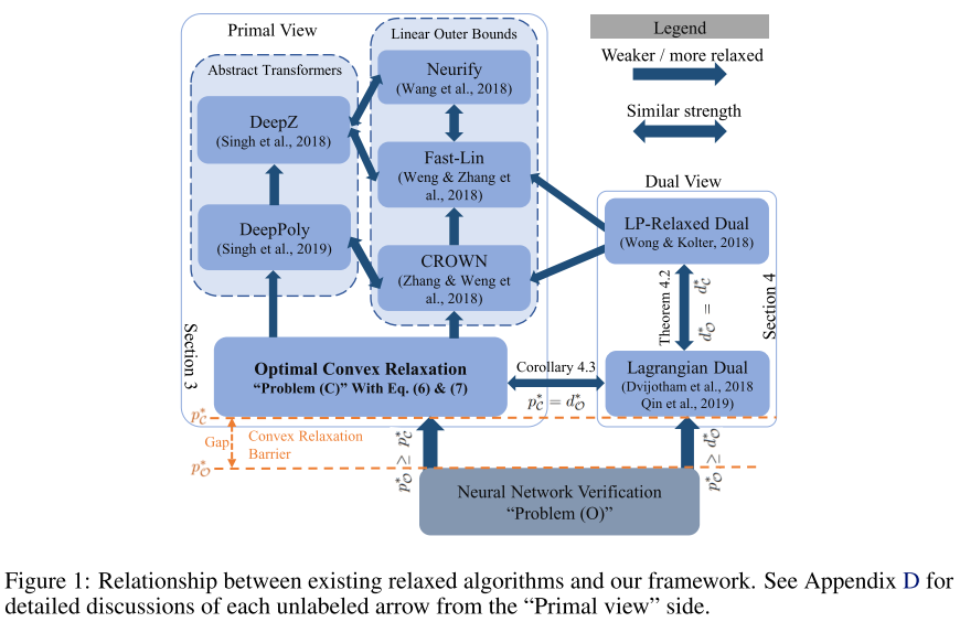
Verification algorithms fall into two categories: exact verifiers that run in exponential time and relaxed verifiers that are efficient but incomplete.

(i) in terms of lower bounding the minimum $l_{\infty}$ adversarial distortion, the optimal layer-wise convex relaxation only slightly improves the lower bound found by Wong and Kolter [2018], especially when compared with the upper bound provided by the PGD attack, which is consistently 1.5 to 5 times larger;

(ii) in terms of upper bounding the robust error, the optimal layer-wise convex relaxation does not significantly close the gap between the PGD lower bound (or MILP exact answer) and the upper bound from Wong and Kolter [2018]

Problem

A classification neural network $f:\R^n\to\R^K$ with $f_i(x)$ as the $i$th logit is considered adversarially robust with respect to an input $x$ and its neighborhood $\mathcal{S}_{in}(x)$ if

It ensures that for the most perturbed example in the attack space, the second largest logit is still smaller than the largest, i.e. correct, logit.

Assume that the neighborhood $\mathcal{S}_{in}(x^{nom})$ is a convex set (e.g. $\mathcal{S}_{in}(x^{nom})=\{x:||x-x^{nom}||_\infty\le\epsilon\}$, the $l_{\infty}$-ball) and $f(x)$ is an $L$-layer feedforward NN.

Denoting $\{0,1,\dots,L-1\}$ as $[L]$ and $\{x^{(0)},x^{(1)},x^{(L-1)}\}$ as $x^{[L]}$, the $f(x)$ is defined as

in which, $x^{(l)}\in\R^{n^{(l)}},z^{(l)}\in\R^{n_z^{(l)}},x^{(0)}:=x\in\R^{n^{(0)}}$ is the input, $\bold{W}^{(l)}\in\R^{n_z^{(l)}\times n^{(l)}}$ and $b^{(l)}\in\R^{n_z^{(l)}}$ are the weight matrix and bias vector of the $l$th linear layer, and $\sigma^{(l)}:\R^{n_z^{(l)}}\to\R^{n^{(l+1)}}$ is a non-linear activation function.

Convex relaxation from the primal view

Consider the following optimization problem $\mathcal{O}(c,c_0,L,\underline{z}^{[L]},\overline{z}^{[L]})$:

The optimization domain $\mathcal{D}$ is

i.e. the set of activations and preactivations satisfying the bounds.

If $c^\top=\bold{W}_{i^{nom}}^{(L)}-\bold{W}_i^{(L)},c_0=b_{i^{nom}}^{(L)}-b_i^{(L)},\overline{z}^{[L]}=\infty$, then $\mathcal{O}$ is equivalent to the original optimization problem. The minimal of this problem is denoted as $p_{\mathcal{O}}^*$.

When we have better information about the valid bounds of $z^{(l)}$, we can significantly narrow donw the optimization domain and achieve tighter solutions when we relax the nonlinearities:

• Obtaining lower and upper bounds by solving sub-problems

  It's widely used but not efficient.

• Convex relaxation in the primal space

  The non-convex equality constraint $x^{(l+1)}=\sigma^{(l)}(z^{(l)})$ can be relaxed to convex inequality constraints, i.e. the optimization problem $\mathcal{C}$:

  $$\min_{(x^{[L+1]},z^{[L]})\in\mathcal{D}}c^\top x^{(L)}+c_0\\ \text{s.t. }z^{(l)}=\bold{W}^{(l)}x^{(l)}+b^{(l)},\underline{\sigma}^{(l)}(z^{(l)})\le x^{(l+1)}\le\overline{\sigma}^{(l)}(z^{(l)}),\forall l\in[L]$$

  where $\overline{\sigma}^{(l)}(z)$ and $\underline{\sigma}^{(l)}(z)$ are convex, satisfying $\underline{\sigma}^{(l)}(z^{(l)})\le \sigma^{(l)}(z^{(l)})\le\overline{\sigma}^{(l)}(z^{(l)})$ for $\underline{z}^{(l)}\le z\le \overline{z}^{(l)}$. The minimum of $\mathcal{C}$ is denoted by $p_{\mathcal{C}}^*$, and $p_{\mathcal{C}}^*\le p_{\mathcal{O}}^*$.

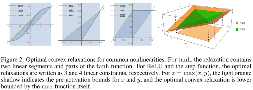
• The optimal layer-wise convex relaxation

  The optimal layer-wise convex relaxation, i.e.

  • $\underline{\sigma}_{opt}(z)$, the greatest convex function majored by $\sigma$.
  • $\overline{\sigma}_{opt}(z)$, the smallest concave function majoring $\sigma$.

  The corresponding optimal relaxed problem is denoted as $\mathcal{C}_{opt}$ with its objective as $p_{\mathcal{C}_{opt}}^*$.

• Greedily solving the primal with linear bounds

  The objective $p_{\mathcal{C}_{opt}}^*$ can be greedily bounded in a layer-by-layer manner when there are exactly one linear upper bound and lower bound for each nonlinear layer in $\mathcal{C}$, i.e.

  $$\overline{\sigma}^{(l)}(z^{(l)}):=\overline{a}^{(l)}z^{(l)}+\overline{b}^{(l)},\underline{\sigma}^{(l)}(z^{(l)}):=\underline{a}^{(l)}z^{(l)}+\underline{b}^{(l)}$$

  Since each layer is linearly bounded, the linear bounds of $z^{(L)}$ with respect to the input $x^{(0)}$ can be recursively acquired.

Intuitively, the convex relaxation expands the attack space to include those for networks with activations in between the higher and lower activation bounds.

Convex relaxation from the dual view

Strong duality for the convex relaxed problem

The Lagrangian dual for problem $\mathcal{C}$ with dual variables introduced is

by weak duality [Boyd and Vandenberghe, 2004]

Theorem 4.1 ($p_{\mathcal{C}}^*=d_{\mathcal{C}}^*$). Assume that both $\underline{\sigma}^{(l)}$ and $\overline{\sigma}^{(l)}$ have a finite Lipschitz constant in the domain $[\underline{z}^{(l)},\overline{z}^{(l)}]$ for each $l\in [L]$. Then strong duality holds between $\mathcal{C}$ and the weak duality.

The dual form is the standard Lagrangian dual form for the relaxed problem.

The optimal layer-wise dual relaxation.

The Lagrangian dual of the original $\mathcal{O}$ is (first proposed by Dvijotham et al. [2018b])

by weak duality

Theorem 4.2 ($d_{\mathcal{O}}^*=d_{\mathcal{C}_{opt}}^*$) Assume that the nonlinear layer $\sigma^{(l)}$ is non-interactive and the optimal layer-wise relaxation $\underline{\sigma}_{opt}^{(l)}$ and $\overline{\sigma}_{opt}^{(l)}$ are defined in (6). Then the lower bound $d_{\mathcal{C}_{opt}}^*$ provided by the dual of the optimal layer-wise convex-relaxed problem and $d_{\mathcal{O}}^*$ provided by the dual of the original problem are the same.

Theorem 4.1 implies that the primal relaxation ($\mathcal{C}$) and the two kinds of dual relaxations, (9) and (11), are all blocked by the same barrier.

Corollary 4.3 ($p_{\mathcal{C}_{opt}}^*=d_{\mathcal{O}}^*$) Suppose the nonlinear activation functions $\sigma^{(l)}$ for all $l\in[L]$ are among the following: ReLU, step, ELU, sigmoid, tanh, ploynomials and max pooling with disjoint windows. Assume that $\underline{\sigma}_{opt}^{(l)}$ and $\overline{\sigma}_{opt}^{(l)}$ are defined in (6), respectively. Then we have that the lower bound $p_{\mathcal{C}_{opt}}^*$ provided by the primal optimal layer-wise relaxation $\mathcal{C}$ and $d_{\mathcal{O}}^*$ provided by the dual relaxation (11) are the same.

Greedily solving the dual with linear bounds

When the relaxed bounds $\underline{\sigma}$ and $\overline{\sigma}$ are linear, the dual objective can be lower bounded as below:

The dual variables are determined by a backward propagation:

I don't get it....

Optimal LP-relaxed Verification

We showed the existence of a barrier, $p_{\mathcal{C}}^*$,that limits all such algorithms. Is this just theoretical babbling or is this barrier actually problematic in practice?

No bounds get higher than $p_{\mathcal{C}}^*$,thus it's a barrier.

To exactly solve the tightest LP-relaxed verification problem of a ReLU network, two steps are required:

1. Obtaining pre-activation bounds

   Obtaining the tightest pre-activation upper and lower bounds of all the neurons in the NN, excluding those in the last layer.

   This is done by solbing sub-problems of the original problem $\mathcal{C}$. Given a NN with $L_0$ layers, for each layer $l_0\in[L_0]$, obtain a lower (resp. upper) bound $\underline{z}_{j}^{(l_0)}$ (resp. $\overline{z}_{j}^{(l_0)}$) , for all neurons $j\in[n^{(l_0)}]$, the followings are done by setting in $\mathcal{C}$:

   $$L\gets l_0,c^\top\gets \bold{W}^{(l_0)}_{j,:}(\text{resp. } c^\top\gets -\bold{W}_{j,:}^\top),c_0\gets b_j^{(l_0)}(\text{resp. }c_0\gets -b_{j}^{(l_0)})$$

   and the exact optimum is computed.

   This is solved in parallel.

   Indeed, we design a scheduler to do so on a cluster with 1000 CPU-nodes.

2. Solving the LP-relaxed problem for the last layer

   Solving the LP-relaxed verification problem exactly for the last layer of the NN.

   With the upper and lower bounds acquired previously, the LP in $\mathcal{C}$ for all $j\in[n^{(L_0)}]\backslash \{j^{nom}\}$ can be obtained by

   $$L\gets L_0,c^{\top}\gets\bold{W}_{j^{nom},:}^{(L_0)}-\bold{W}_{j,:}^{(L_0)},c_0\gets b_{j^{nom}}^{(L_0)}-b_{j}^{(L_0)}$$

   and the exact minimum is computed.

   Here, $j^{nom}$ is the true label of the data point $x^{nom}$.

   We can certify the network is robust around $x^{nom}$ iff the solutions of all such LPs are positive, i.e. we cannot make the true class logit lower than any other logits.

Experiments

We conduct two experiments to assess the tightness of LP-ALL:

1) finding certified upper bounds on the robust error of several NN classifiers,

2) finding certified lower bounds on the minimum adversarial distortion $\epsilon$ using different algorithms.

All experiments are conducted on MNIST and/or CIFAR-10 datasets.

We conduct experiments on a range of ReLU-activated feedforward networks. MLP-A and MLP-B refer to multilayer perceptrons: MLP-A has 1 hidden layer with 500 neurons, and MLP-B has 2 hidden layers with 100 neurons each.

We run experiments on a cluster with 1000 CPU-nodes. The total run time amounts to more than 22 CPU-years.

It's computational expensive....

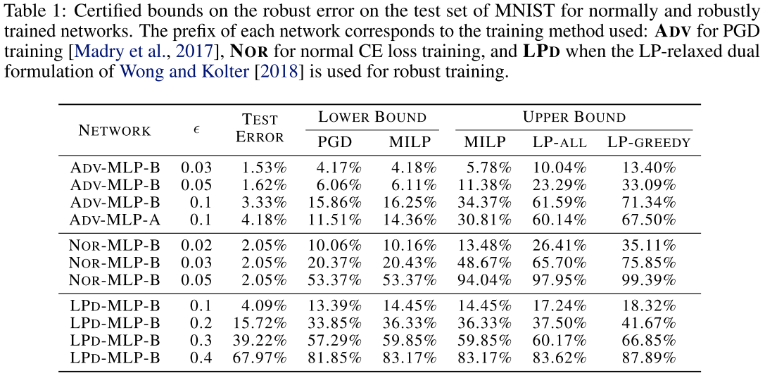
For all NORmally and ADV-trained networks, we see that the certified upper bounds using LP-GREEDY and LP-ALL are very loose when we compare the gap between them to the lower bounds found by PGD and MILP.

We are interested in searching for the minimum adversarial distortion $\epsilon$, which is the radius of the largest $l_{\infty}$ ball in which no adversarial examples can be crafted.

Since solving LP-ALL is expensive, we find the -bounds only for ten samples of the MNIST and CIFAR-10 datasets.

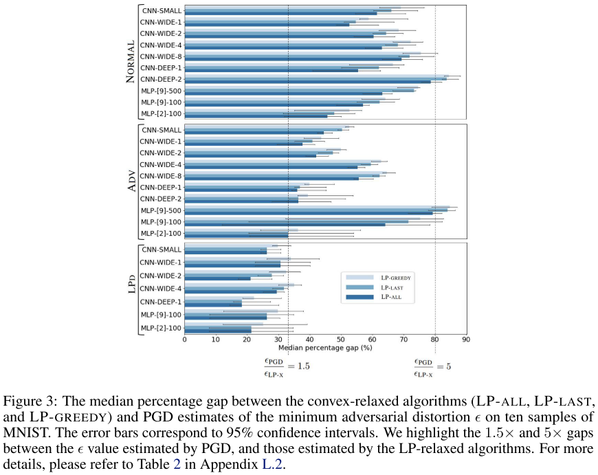
On MNIST, the results show that for all networks trained NORmally or via ADV, the certified lower bounds on are 1.5 to 5 times smaller than the upper bound found by PGD

This indicates that although PGD cannot find an adversarial example in the smaller radius but the adversarial examples exist in a smaller radius, verified by the robust verification.

Then we performed extensive experiments to show that even the optimal convex relaxation for ReLU networks in this framework cannot obtain tight bounds on the robust error in all cases we consider here. Thus any method will face a convex relaxation barrier as soon as it can be described by our framework

In so far as the ultimate goal of robustness verification is to construct a training method to lower certified error, this barrier is not necessarily problematic — some such method could still produce networks for which convex relaxation as described by our framework produces accurate robust error bounds.

Inspirations

This paper provides a large amount of mathematical equations and notations, which are a little overwhelmed, a smaller portion of them will be favored.

The conculsion indicates that all the methods with convex relaxation are barriered by the optimal convex relaxation, thus none of them succeeds in finding the real lower bound, but in practice, this gap so far still provide accurate robust error bounds.

It's clear that the method proposed can be improved computationally, otherwise it will never be a prevailing method.

Semantify-NN - CVPR 2020

Code: https://github.com/JeetMo/SemantifyNN

Jeet Mohapatra, Tsui-Wei (Lily)Weng, Pin-Yu Chen, Sijia Liu, Luca Daniel. Towards Verifying Robustness of Neural Networks Against A Family of Semantic Perturbations. CVPR 2020. arXiv:1912.09533

To bridge this gap, we propose Semantify-NN, a model-agnostic and generic robustness verification approach against semantic perturbations for neural networks.

They propose a Semantic Perturbation layer that can be inserted into the input layer of any given model, which is capable of verifying the robustness of model under semantic perturbations.

Given a data sample $x$ and a trained DNN, the primary goal of verification tools is to provide a “robustness certificate” for verifying its properties in a specified threat model.

Robustness certification

Given a threat model $\mathcal{A}$, with which the attack space for an input data sample $x$ is $\Omega_\mathcal{A}(x)$, equipped with a distance function $d_{\mathcal{A}}$ to measure the magnitude of the perturbation, the problem of robustness certification is to find the largest $\delta$ such that

where $f$ is a trained $K$-class classifier and $f_j(\cdot)$ is the confidence of the $j$-th class ($j\in\{1,2,\dots,K\}$), and $c$ is the predicted class of un-perturbed input data $x$.

In short, it aims to find the largest magnitude bound under a certain threat model that every perturbation permitted fails to change the classification result.

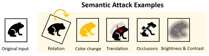
Semantic perturbation

In general, semantic adversarial attacks craft adversarial examples by tuning a set of parameters governing semantic manipulations of data samples, which are either explicitly specified (e.g. rotation angle) or implicitly learned (e.g. latent representations of generative models).

Continuously parameterized semantic perturbations cannot be enumerated.

This name is tricking, the semantic perturbations are basically manipulations of the image that preserve the semantic meaning of the image. Actually a few years ago, this may be seen as a method to test the generalization of models.

For an attack space $\Omega_{\mathcal{A}}^k$, there exists a function

such that

In which

• $X$ is the pixel space (i.e. the raw image)

• $I_i$ denotes a set of feasible semantic operations

• $\epsilon_i$ specify semantic operations selected from $I_i$

• $k$ denotes the dimension of semantic attack

  $$\epsilon^k=(\epsilon_1,\epsilon_2,\dots,\epsilon_k)\\ I^k=I_1\times\cdots\times I_k$$

•  

For example, $\epsilon_i$ can describe some human-interpretable characteristic of an image, such as translations shift, rotation angle, etc.

Semantic attacks can be divided into two categories

• Discretely parameterized perturbations

  (translation, occlusions, etc.)

• Continuously parameterized perturbations

  (color changes, brightness, contrast, spatial transformations, etc.)

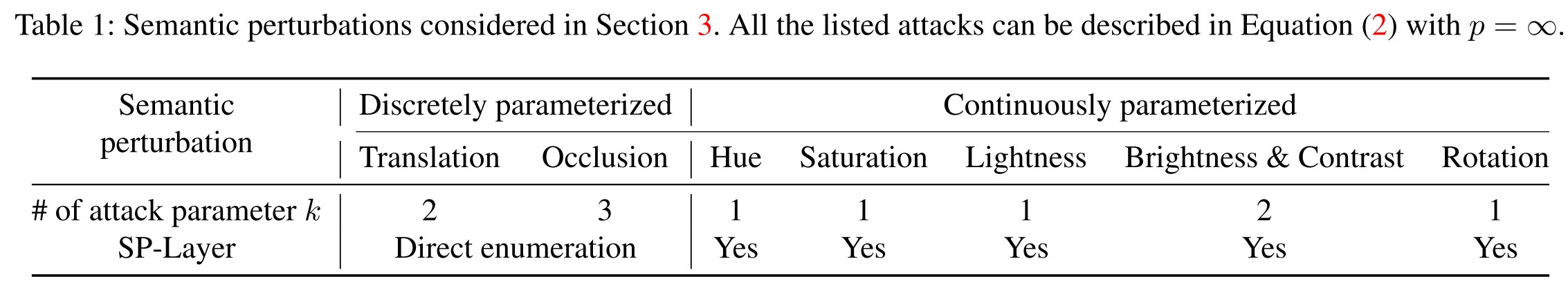
Discretely Parameterized Semantic Perturbation

• Translation

  It's a 2-dimensional semantic attack with two parameters denoting the relative positions of left-uppermost pixel of perturbed image to the original image, i.e. $I_1=\{0,1,\dots,r\},I_2=\{0,1,\dots,t\}$ for an image of size $r,t$.

• Occlusion

  It can be expressed by a 3-dimensional attack with three parameters, i.e. the coordinates of the left-uppermost pixel of the occlusion patch and the size of the patch.

SP-layers (Continuously Parameterized Semantic Perturbation)

In this case, the semantic perturbation parameters are continuous values, i.e. $I^k\sub \R^k$.

They propose to add semantic perturbation layers (SP-layers) to the input layer for efficient robustness verification.

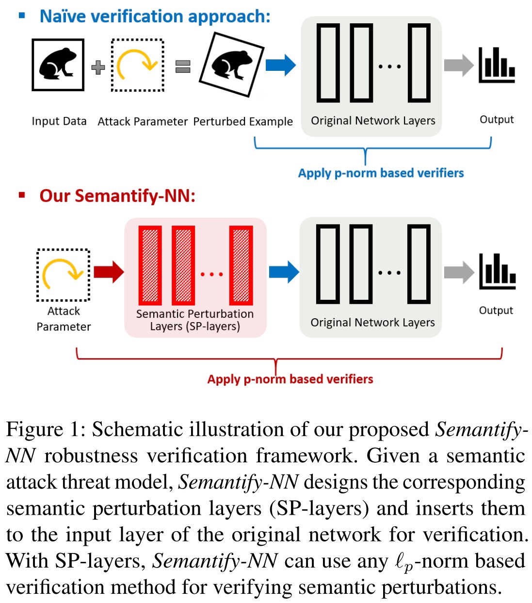
Substituting $g_x(\epsilon^k)=g(x,\epsilon^k)$, the verification problem becomes

Reforming the network as $f^{sem}=f\circ g_x$, it further becomes

which shares similar form with that for $l_p$-norm perturbations, but now on the semantic space $I^k$.

Overall, the SP-layers work as a parameterized input transformation function from the semantic space to RGB space used for further predictions.

Instantiations of SP-layers

Hue

Two colors with the same hue are generally considered as different shades of a color, like blue and light blue.

The hue is represented on a scale of $0-360^\circ$ and for convenience they rescale it to the range $[0,6]$, thus there is

In which,

and

where $V=(1-|(h^\prime\mod 2)-1|)$.

For $0\le h^{\prime}\le 6$, the above can be reduced with a ReLU activation, i.e. $\sigma_i(x)=\text{ReLU}(x-i)$ to a hidden layer connecting from hue space to original RGB space:

Intriguing, thus it becomes a layer of networks.

Saturation

This value corresponds to the colorfulness of the picture, with a saturation of 0, the picture becomes gray-scale.

In which

and

Hence it also becomes a layer of network.

Lightness

This property corresponds to the perceived brightness of the image where a lightness of 1 gives us white and a lightness of 0 gives us black images.

In which

and

Another layer of network!

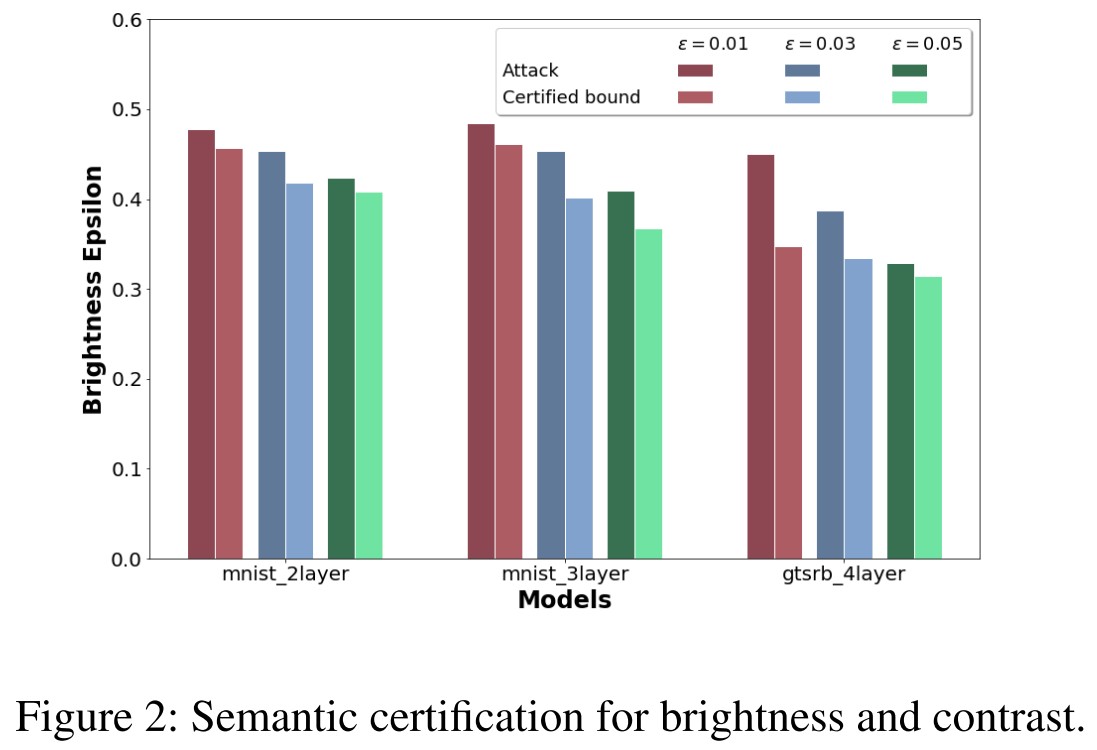
Brightness and contrast

With the brightness controlled by $\epsilon_b$ and contrast controlled by $\epsilon_c$, this layer is

Rotation

Rotation can be expressed as a 1-dimension attack parameterized by the rotation angle $\theta$. They consider rotations at the center of the image with the boundaries being extended to the area outside the image.

For the value of output pixel at position $(i,j)$, denoted as $x_{i,j}^\prime$, after rotation by $\theta$, it's acquired by

In which

and $k,l$ range over all possible values.

This part is a little weird.

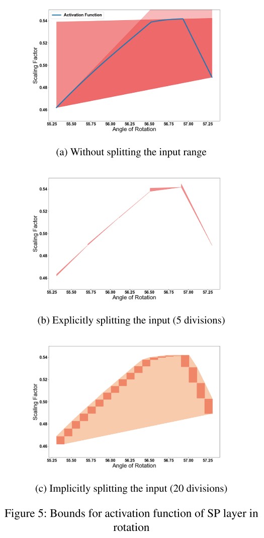
For a single pixel at $(k,l)$ on the original image, the scaling factors for its influence on the output pixel at position $(i,j)$ is given by

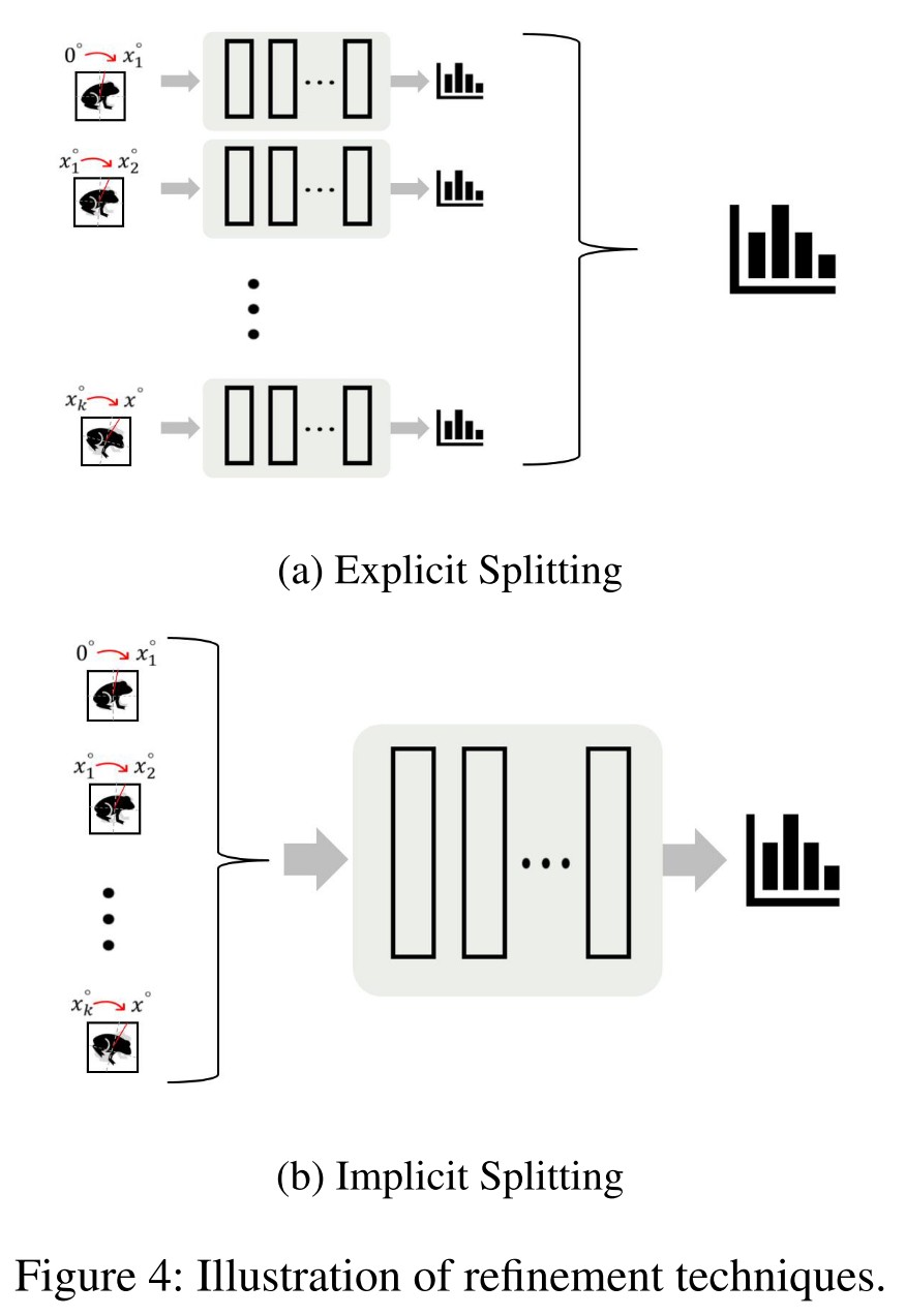
It's highly non-linear and it's 0 for most $\theta$ and for a very small range of $\theta$, it takes non-zero values which can go up to 1.

This makes naive verification infeasible and one idea is to use Explicit Input Splitting (split the range of angles into small parts), but it's still computationally infeasible for a large number of splitsim.

To balance this trade-off, we propose a new refinement technique named as implicit input splitting.

Input space refinement for Sematify-NN

Theorem 3.1. Given an image $x$, if we can verify that a set $S$ of perturbed images $x^\prime$ is correctly classified for a threat model using one certification cycle, then we can verify that every perturbed image $x^\prime$ in the convex hull of $S$ is also correctly classified, where the convex hull in the pixel space.

Here one certification cycle means one pass through the certification algorithm sharing the same linear relaxation values.

As a result, we can split the original interval into smaller parts and certify each of them separately in order to certify the larger interval.

Intuitively, since the minimizer of the output space for the union of intervals is one of the minimizers for each intervals, thus the minimum requirement still holds for the union if it holds for every interval.

We find that we are unable to get good verification results for datasets like MNIST and CIFAR-10 without increasing the number of partitions to very large values (≈ 40, 000).

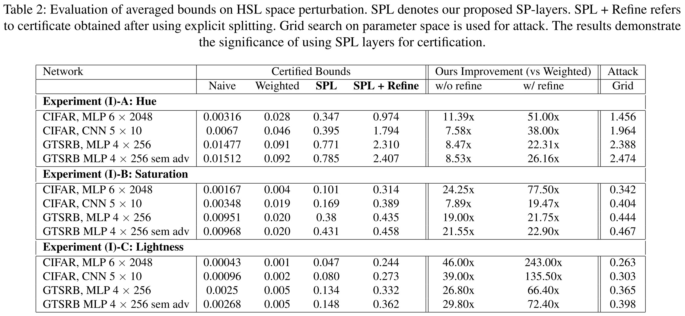
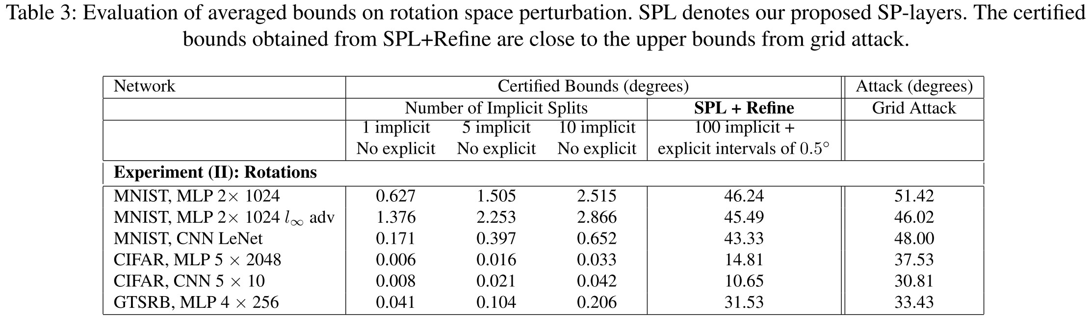
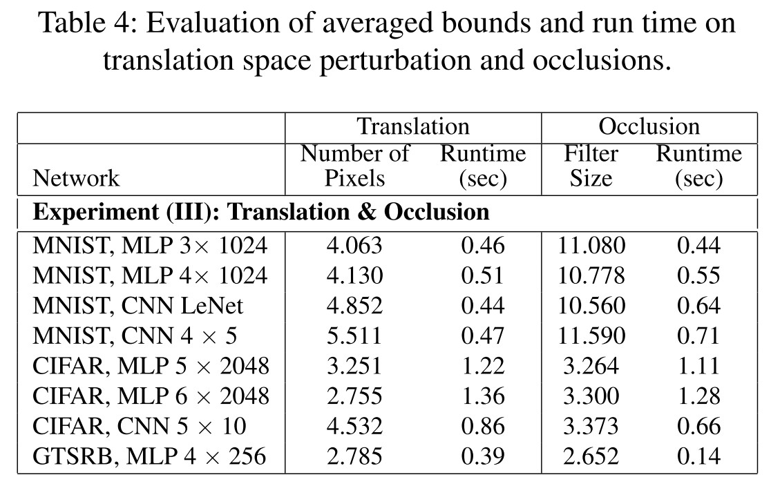
Experiments

Inspirations

The so-called semantic perturbation seems familiar and some years ago, they were used to test the generalization of models in face of corruptions, translations and rotations. Specially, CNN used to be claimed to be translational invariant and rotational invariant.

This paper reformulates the semantic perturbations into the form of an handcrafted neural network that transforms the parameter space into the image space, defining the attack space implicitly. This structure and intuition sounds very familiar, if we refer the parameter space as latent space and view the Semantify-NN as a generator and the classifier as a discriminator, the whole thing becomes a Generative Adversarial Nets, i.e. GAN, but with a handcrafted generator and a multi-class discriminator.

Based on this resembling, I think someone will soon use a GAN to solve this problem.

Adversarial Training + Verification

COLT (Convex Layerwise Adversarial Training) - ICLR 2020

Code: https://github.com/eth-sri/colt

Paper: https://openreview.net/forum?id=SJxSDxrKDr

Mislav Balunovic, Martin Vechev. Adversarial Training and Provable Defenses: Bridging the Gap. ICLR 2020.

They propose to train the network with both a verifier and an adversary.

The overall procedure is:

1. The verifier produces a convex relaxation of all possible intermediate vector outputs in the neural network to certify a property (e.g. robustness) of the network.
2. An adversary searches over this (intermediate) convex region in order to find a latent adversarial example, i.e. a concrete intermediate input contained in the relaxation that when propagated through the network causes a misclassification which prevents verification.
3. The resulting latent adversarial examples are now incorporated into our training scheme using adversarial training.

Threat model and settings

In the threat model they consider, an adversary is allowed to transform an input $\bold{x}\in\R^{d_0}$ into any point from a convex set $\Bbb{S}_0(\bold{x})\sube\R^{d_0}$.

A convex set is a set that for every two elements in this set, the weighted combination of them is still an element in the set.

This set $\Bbb{S}_0$ can capture a wide range of specifications, including:

• $L_p$ perturbations
• Geometric transformations
• Semantic perturbations
• Camera imaging

For the $L_{\infty}$ perturbations, this specification of convex set is

A neural network of $k$ layers parameterized with $\theta$ is

In which, $h_{\theta}^i:\R^{d_{i-1}}\to\R^{d_i}$ denotes a transformation applied at a hidden layer $i$. The function of a part of the network from layer $i$ to the final layer $k$ is denoted as

The goal of verification is to prove a property on the output of the neural network, encoded via a linear constraint:

in which, $c$ and $d$ are property specific vector and scalar values respectively.

The standard approach to train a model $h_{\theta}$ to satisfy this constraint is to define a surrogate loss $\mathcal{L}$ and solve the following min-max optimization problem:

Based on the approximation used to solve the inner maximization, there are two families of techniques:

• Adversarial Training

  It replaces the maximum loss with a lower bound obtained using an adversarial attack. The PGD-based adversarial training is empirically robust but without guarantees.

• Provable Defenses

  It replaces the maximum loss with a computed upper bound, hence providing guarantees on the robustness of the resulting network inside the threat model.

  But the upper bound is computed using relaxation, which is typically not tight, and the way the bound is computed is also significantly more complex.

Certification via convex relaxations

The set of possible intermediate concrete vectors at layer $i$, i.e.

which can be obtained by propagating vector $\bold{x}\prime\in\Bbb{S}_0(\bold{x})$ through the network layer by layer.

With the difficulties to compute the set $\Bbb{S}_i(\bold{x})$, it's standard to approximate it via a convex relaxation $\Bbb{C}_i(\bold{x})$. Thus the input approximation is $\Bbb{C}_0(\bold{x})=\Bbb{S}_0(\bold{x})$, since it's already convex.

For any set $\Bbb{D}\sube\R^{d_{i-1}}$, the set obtained using a convex relaxation of the transformation in layer $i$, denoted as $g_{\theta}^i(\Bbb{D})$ is convex, and there exists $h_{\theta}^i(\Bbb{D})\sube g_{\theta}^i(\Bbb{D})$.

So a convex relaxation of the intermediate vectors can be recursively defined as

Since $\Bbb{S}_k(\bold{x})\sube \Bbb{C}_k(\bold{x})$, it is sufficient to check if all output vectors in $\Bbb{C}_k(\bold{x})$ satisfy the linear constraint to ensure that all vectors in $\Bbb{S}_k(\bold{x})$ satisfy the constraint.

But it's possible that there exists an intermediate vector $\bold{x}_i^\prime$ in layer $i$ such that $c^\top h_{\theta}^{i+1:k}(\bold{x}_i^\prime)+d\ge 0,\bold{x}_i^\prime\in\Bbb{C}_i(\bold{x})\backslash \Bbb{S}_i(\bold{x})$, leading the failure of certification.

It's possible that the original set is satisfactory while the convex relaxation violates the property.

These points are referred as latent adversarial examples.

Convex Layerwise Adversarial Training

Our key observation is that the two families of defense methods described earlier are in fact different ends of the same spectrum: methods based on adversarial training maximize the cross-entropy loss in the first convex region $\Bbb{C}_0(\bold{x})$ while provable defenses maximize the same loss, but in the last convex region $\Bbb{C}_k(\bold{x})$.

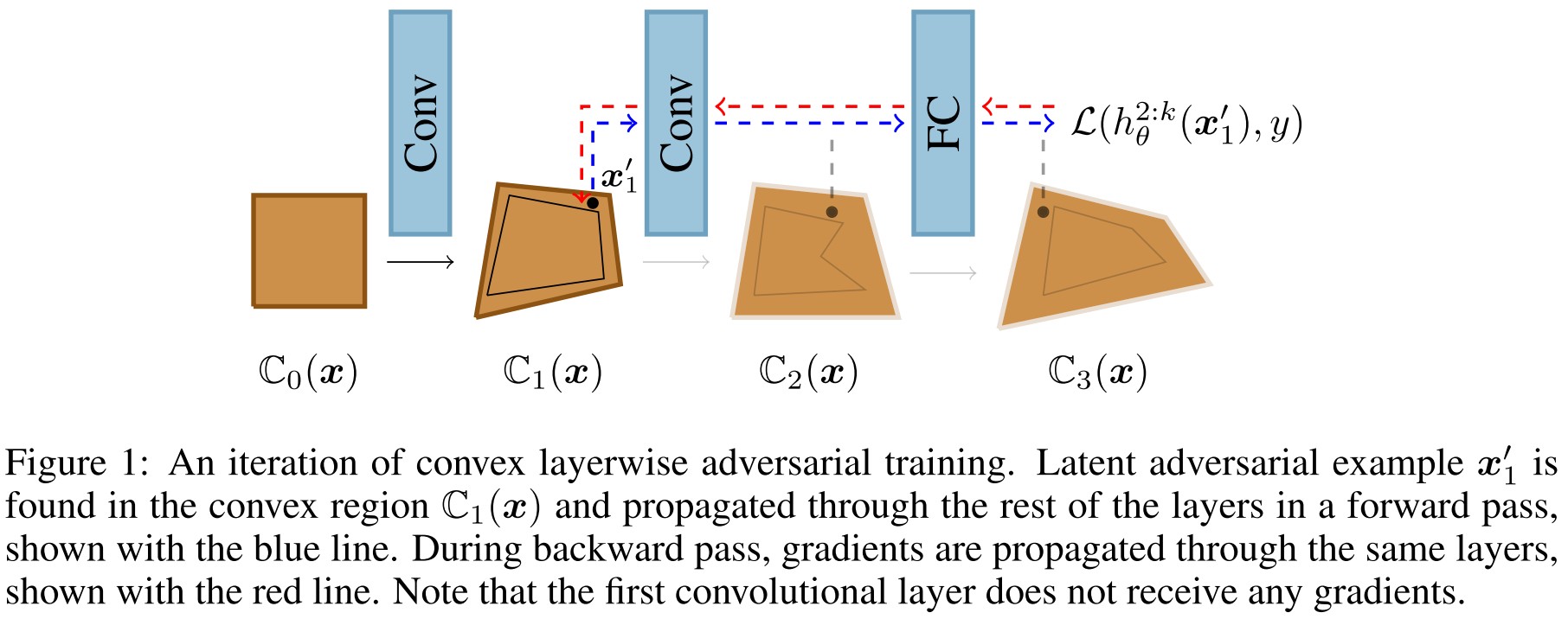
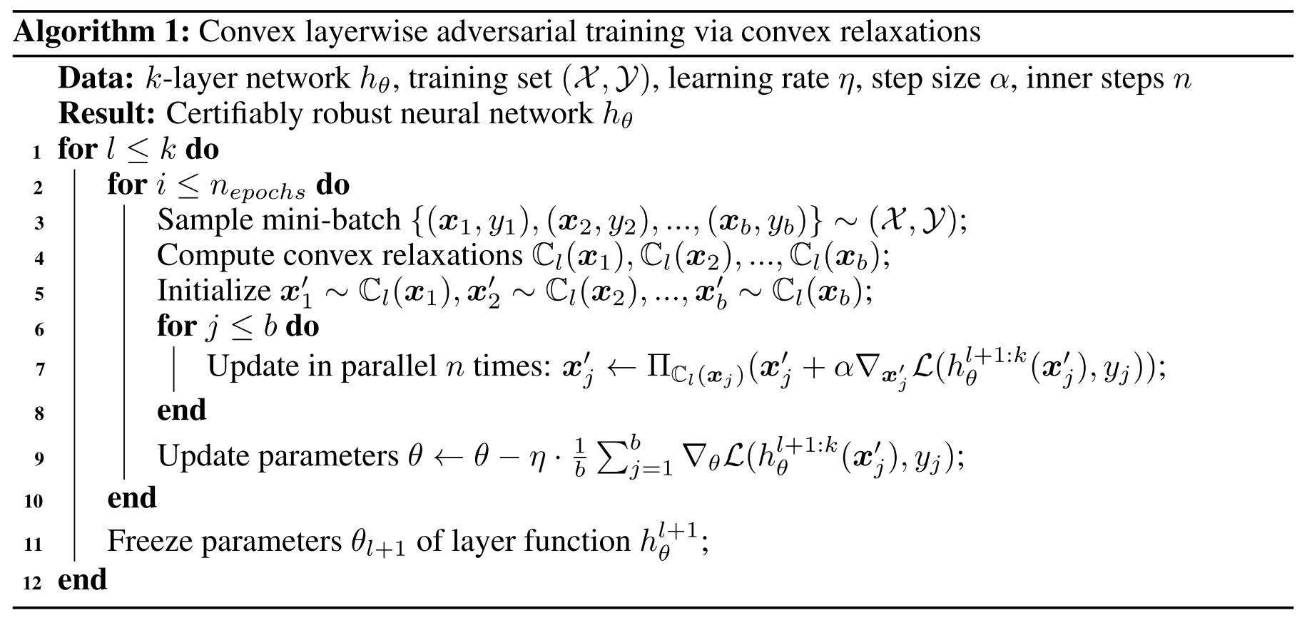
They propose COLT as a combination, the concrete steps are as follows:

1. Conduct an iteration of standard adversarial training in $\Bbb{C}_0(\bold{x})$.
2. Freeze the first layer, find a concrete point in $\Bbb{C}_1(\bold{x})$ to maximize the loss and then backpropagate the update the weights from the second layer to the last one.
3. From the second to the last layer, iteratively conduct the same procedure in step 2.

At the $l$-th step, COLT solves the following min-max optimization problem:

which is equivalent to the standard form when $l=0$, as well as $\Bbb{C}_0(\bold{x})=\Bbb{S}_0(\bold{x})$.

Calculate convex approximation using linear relaxation

A linear relaxation of $\Bbb{S}_l(\bold{x})$ can be represented by a set

The vector $\bold{a}_l$ represents the center of the set and the matrix $A_l$ represents the affine transformation of the hypercube $[-1,1]^{m_i}$. This representation is also known as zonotope abstraction.

A convex relaxation can be represented by an affine transformed and shifted standard hypercube.

The initial convex set will be represented with $\bold{a}_0=\bold{x}$ and $A_0=\epsilon I_{d_o}$, and $A_l\bold{e}$ can be computed by performing a chain of matrix-vector multiplications from right to left instead of matrix-matrix multiplications.

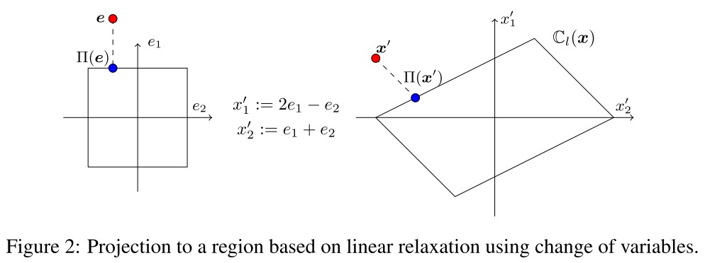
With this representation, the projection of $\bold{x}^\prime$ can be conducted in the spave of $\bold{e}$. The Line 7 of the above algorithm is instantiated with the following operations:

with the clip defined as $clip(t,-1,1):=\min(\max(t,-1),1)$.

Experiments

The certification of the neural networks is conducted using exactly solved convex hulls for each intermediate features.

If training was successful, there should not exist a concrete point $\bold{x}^\prime\in\Bbb{C}_l(\bold{x})$ which, if propagated through the network, violates the correctness property in Equation 1.

We remark that this combination of convex relaxation and exact bound propagation does not fall under the recently introduced convex barrier to certification Salman et al. (2019b).

They evaluate on two architectures (both very small):

• A 4-layer convolutional network: first 3 layers are convolutional layers with filter sizes 32, 32, 128, kernel sizes 3, 4, 4 and strides 1, 2, 2, respectively.
• A 3-layer convolutional network: first 2 layers are convolutional layers with filter sizes 32 and 128, kernel sizes 5 and 4, strides 2 and 2, respectively.

We always compare to the best reported and reproducible results in the literature on any architecture.

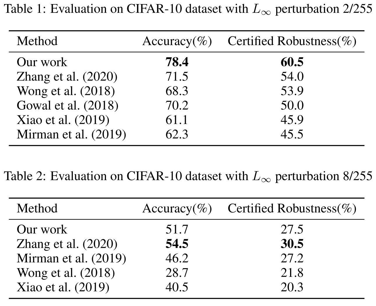
Larger architecture produces the results in Table 1 and smaller architecture produces the results in Table 2.

They also evaluate the latent adversarial robustness.

In this experiment, we are interested in robustness of a model against latent adversarial attacks during each stage of the training. To perform this experiment, after each stage of the training we stored the intermediate model and ran latent adversarial attack on these models, on each of the layers.

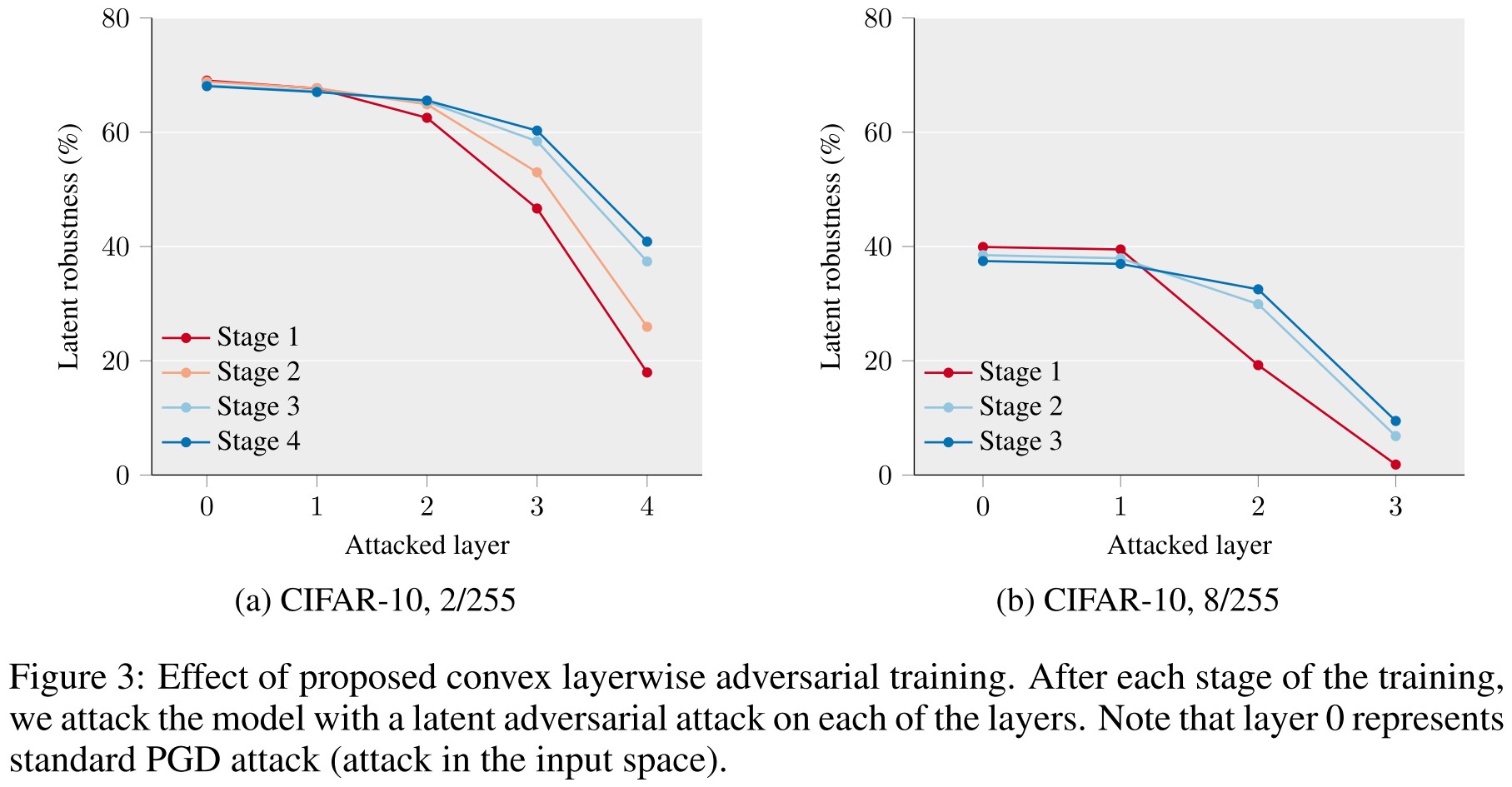
Using convex layerwise adversarial training, the model progressively becomes robust to perturbations in the deeper layers.

It seems that the deeper layer is always less robust than the more shallow layer.

They also evaluate on MNIST and SVHN, both using the smaller architecture.

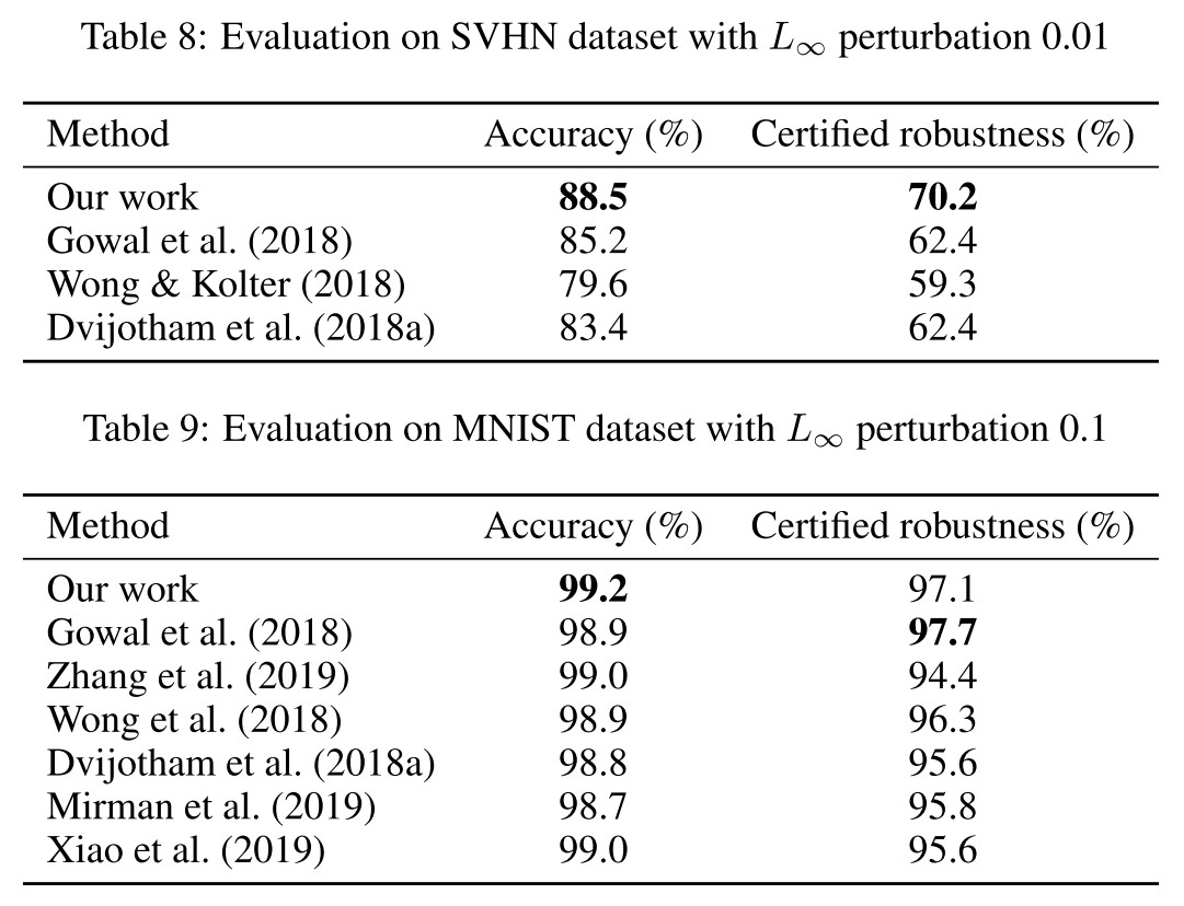
We believe that instantiating our method with a convex relaxation that is more memory friendly than what we used would likely yield better results in this experiment.

Inspirations

This paper presents COLT, a new method combining the verification and adversarial training. To me, it's basically layerwise adversarial training on feature map, but with a convex relaxation of the set of feature maps, But it's two computationally expensive, and it's expected to see a work trying to fasten it.

Another inspiration is that, since adversarial training from feature maps to the predictions works, is it possible to conduct adversarial training from input to feature maps? (Adversarial Logit Pairing conduct it from input to logits and TRADES combine standard training with Adversarial Logit Pairing, it seems that no one has tried to do it.)