Advances along Adversarial Training - 1

By LI Haoyang 2020.10.26

Content

The prevailing defense method is called adversarial training. Theoretically, a min-max optimization is formulated with the idea of adversarial training to train a robust model,i.e. adversarial training, aiming to solve the following problem:

The inner formulation searches an optimal perturbation in allowed perturbations $\cal{S}$ and the outer formulation searches an optimal parameter $\theta$ to minimize the loss function respect to the perturbed example.

However, even the model trained with adversarial training is not highly robust. The defense of adversarial attack is still an unsolved problem.

Adversarial Training

Formulated adversarial training - ICLR 2018

Code: https://github.com/MadryLab/mnist_challenge

Challenge: https://github.com/MadryLab/cifar10_challenge

Aleksander Madry, Aleksandar Makelov, Ludwig Schmidt, Dimitris Tsipras, Adrian Vladu. Towards Deep Learning Models Resistant to Adversarial Attacks. ICLR 2018. arXiv:1706.06083

They want to combine attack and defense into one framework and create a challenge for community to boost further research.

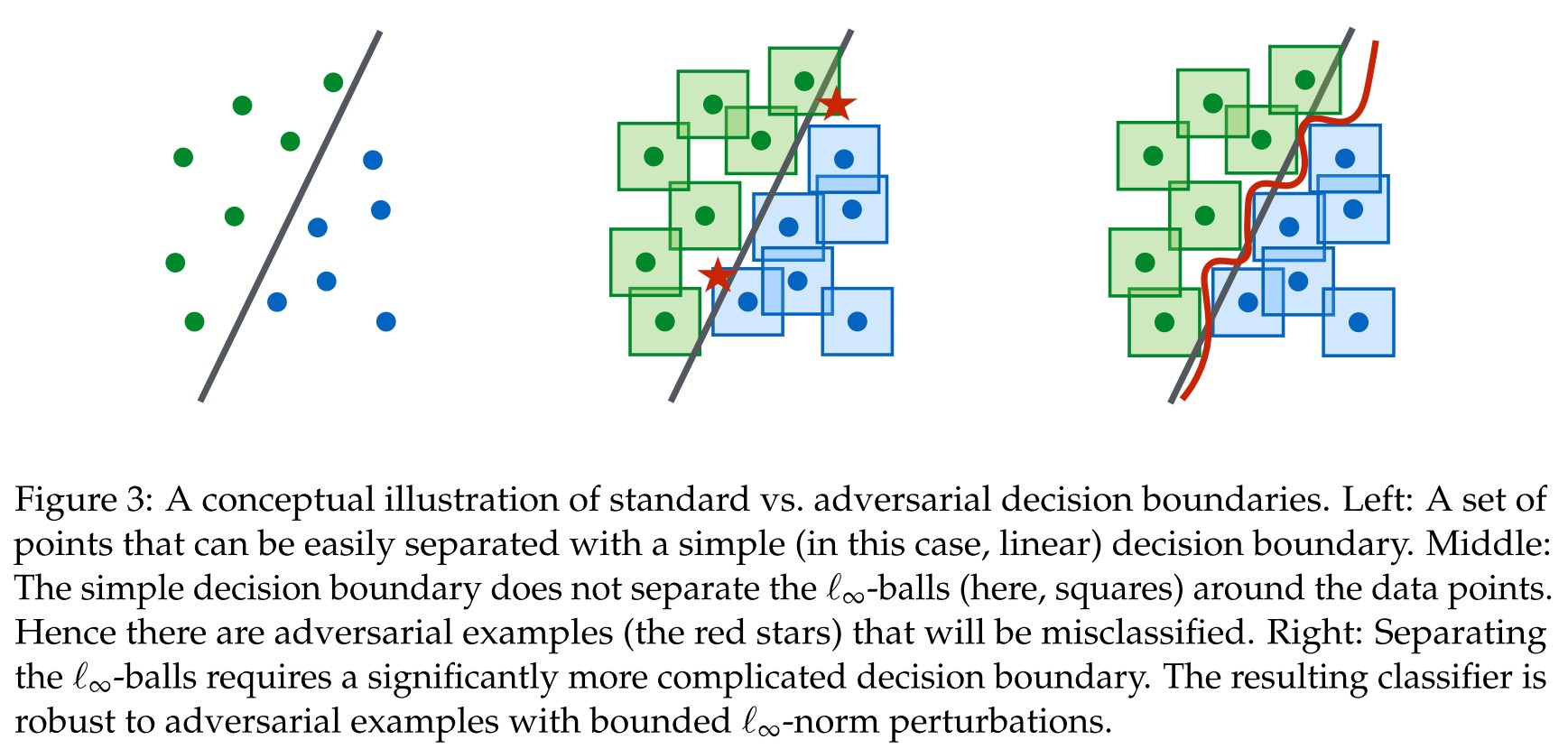
The strategy for defense is still adversarial training. As shown in Figure 3, with adversarial training, the model is able separate the affinities ($l_{\infin}$-balls) of examples.

Problem formulation

The prevailing formulation of the problem of classification is the Empirical Risk Minimization paradigm, which is formulated as:

• $\cal{D}$ is the data distribution over pairs of examples $x\in\Bbb{R}^d$ and corresponding labels $y\in[k]$.
• $\theta\in\Bbb{R}^p$ is the set of model parameters
• $L(x,y,\theta)$ is a suitable loss function

Put the adversary into the problem above, a saddle point (min-max) problem is drawn to formulate the goal of adversarial defense:

• $\cal{S}\subseteq \Bbb{R}^d$ is a set of allowed perturbations
• $\delta$ is the adversarial perturbation

The inner maximization problem aims to find an adversarial version of a given data point $x$ that achieves a high loss. This is precisely the problem of attacking a given neural network.

On the other hand, the goal of the outer minimization problem is to find model parameters so that the “adversarial loss” given by the inner attack problem is minimized.

In short, the problem of defending adversarial attack is formulated into a min-max optimization problem. The adversary adjusts the input to attack the model; while the defender adjusts the parameters to defend the model.

Projected gradient descent

In this paper, PGD is claimed to be the "universal" adversarial attack, and a series of experiments conducted conjecture that:

if we train a network to be robust against PGD adversaries, it becomes robust against a wide range of other attacks as well.

More complete illustration of PGD: Projected Gradient Method and LASSO (Chinese)

Basically, PGD is gradient descent with projection in each step in order to project variable $x_{k}-t_k\nabla f(x_k)$ updated with gradient descent into a feasible region $\cal{C}$:

It is originally written as:

$$x^{t+1}=\prod_{x+\mathcal{S}}(x^t+\alpha sgn(\nabla_xL(\theta,x,y)))$$

with a confusing $\prod$, in which $\prod_{x+\mathcal{S}}$ means projecting $x$ back if $x$ exceeds $x+\mathcal{S}$.

In the problem of generating adversarial examples, the famous FGSM is a one step version of PGD. The PGD is fundamentally the same as I-FGSM referred in other place, which is an iterative version of fast gradient sign method.

Danskin's theorem

However, for the case of continuously differentiable functions, Danskin’s theorem—a classic theorem in optimization—states this is indeed true and gradients at inner maximizers corresponds to descent directions for the saddle point problem

Consider the min-max optimization problem under a single example $x$ and its label $y$ from distribution $\cal{D}$:

Theorem A.1(Danskin). Let $\cal{S}$ be noempty compact topological space and $g:\Bbb{R}^n\times \cal{S}\rightarrow \Bbb{R}$ be such that $g(\cdot,\delta)$ is differentiable for every $\delta\in\cal{S}$ and $\nabla_{\theta}g(\theta,\delta)$ is continuous on $\Bbb{R}^n\times \cal{S}$. Also, let $\delta^{*}(\theta)=\{\delta\in\arg\max_{\delta\in\cal{S}}g(\theta,\delta)\}$.

Then the corresponding max-function

$$\phi(\theta)=\max_{\delta\in\cal{S}}g(\theta,\delta)$$

is locally Lipschitz continuous, directionally differentiable, and its directional derivatives satisfy

$$\phi^{'}(\theta,h)=\sup_{\delta\in\delta^*(\theta)}h^T\nabla_{\theta}g(\theta,\delta)$$

In particular, if for some $\theta\in\Bbb{R}^n$ the set $\delta^*(\theta)=\{\delta_{\theta}^*\}$ is a singleton, then the max-function is differentiable at $\theta$ and

$$\nabla\phi(\theta)=\nabla_{\theta}g(\theta,\delta_{\theta^*})$$

Apply the theorem of Danskin to the problem, the following corollary is induced:

Corollary A.2. Let $\overline{\delta}$ be such that $\overline{\delta}\in \cal{S}$ and is a maximizer for $\max_{\delta}L(\theta,x+\delta,y)$. Then, as long as it is nonzero, $-\nabla_{\theta}L(\theta,x+\overline{\delta},y)$ is a descent direction for $\phi(\theta)=\max_{\delta\in\cal{S}}L(\theta,x+\delta,y)$.

According to Corollary A.2, the outer problem can be solved using normal methods at the optimizer of inner problem.

Performance

There are several observations:

• Capacity alone helps (i.e. larger model is more robust)

• FGSM adversaries don’t increase robustness (the same observation as that in DeepFool).

• Weak models may fail to learn non-trivial classifiers.

  The small capacity of the network forces the training procedure to sacrifice performance on natural examples in order to provide any kind of robustness against adversarial inputs.

• The value of the saddle point problem decreases as we increase the capacity.

• More capacity and stronger adversaries decrease transferability.

Analysis of the robust MNIST classifier

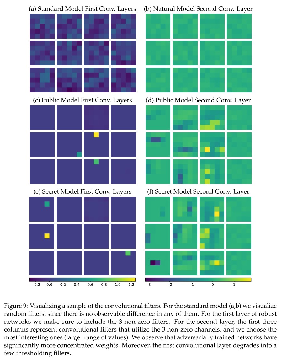
It can be observed that the adversarially trained model has a more sparse parameters than the standard model, which proves that regularization over weights increases robustness as mentioned in Intriguing Properties of Neural Networks

Inspirations

This paper theoretically solves the problem of adversarial example by defining and proving the formulation of defense. The subsequent experiments also prove the potential of this direction.

There are quite a lot of possible work deriving from this paper:

• Domain adaptation - apply this method to domain specific attacks
• Disentangle the defense and normal training - it will be much more useful if the adversarial attack can be defended by adding a separate module to existing models
• Attack the so-called robust model - current attempts have been tried on the open challenge and it's possible
• Improve the robustness - if the illustration depicted by the author is correct, then the robustness is actually gained by overfiting the dense example space expanded by $l_{\infin}$-norm balls. The better performance of larger model also proves the help of overfiting. But the $l_{p}$-norm does not indicate the imperceptibility, so the separating metric itself is flawed and the model is overfiting according to it...

Adversarial Logit Pairing - 2018

Harini Kannan, Alexey Kurakin, Ian Goodfellow. Adversarial Logit Pairing. arXiv preprint 2018 arXiv:1803.06373

We introduce enhanced defenses using a technique we call logit pairing, a method that encourages logits for pairs of examples to be similar.

They propose to pair the logits of adversarial example and corresponding origins in adversarial training.

All previous attempted defenses on ImageNet (Kurakin et al., 2017a; Tramer et al., 2018) report error rates of 99 percent on strong, multi-step white box attacks.

Mixed-minibatch PGD (M-PGD)

Extending the original PGD adversarial training to train on a mixture of clean and adversarial examples, the problem is now formulated as

Logit Pairing

For a model that takes inputs $x$ and computes a vector of logits $z=f(x)$, logit pairing adds a loss

for pairs of training examples $x$ and $x^{'}$, where $\lambda$ is a coefficient determining the strength of the logit pairing penalty.

Adversarial logit pairing (ALP)

Consider a model parameterized with $\bold{\theta}$ trained on a minibatch $\Bbb{M}$ of clean examples $x^{(i)}$ and its corresponding adversarial examples $\tilde{x}^{(i)}$, adversarial logit pairing consists of minimizing the following loss

Clean logit pairing (CLP)

In CLP, the logit is paired between two clean images. The loss to be minimized is

To our surprise, inducing similarity between random pairs of logits led to high levels of robustness on MNIST and SVHN.

Clean logit squeezing

To this end, we tested penalizing the norm of the logits, which we refer to as “logit squeezing” for the rest of the paper. For MNIST, it turned out that logit squeezing gave us better results than logit pairing.

Experiments

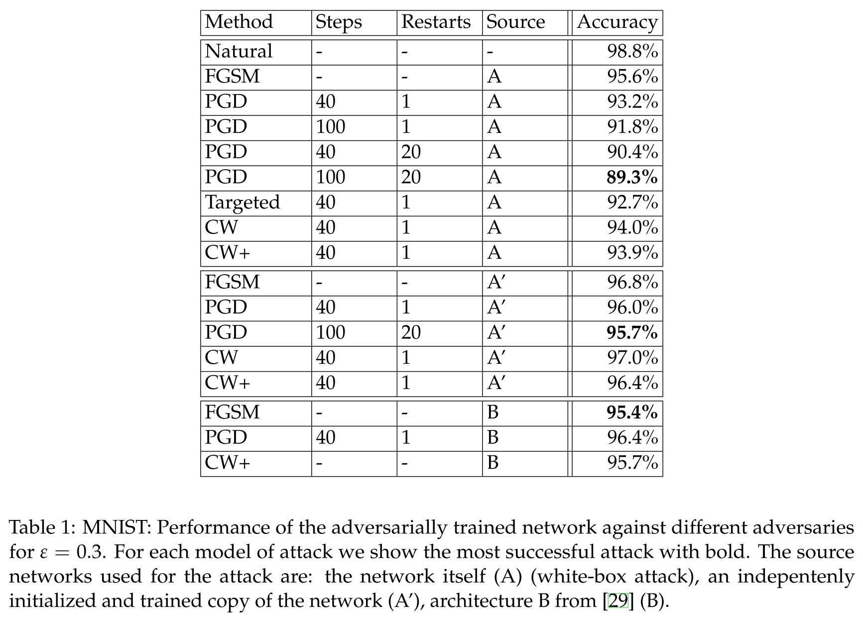
We used the LeNet model as in Madry et al. (2017). We also used the same attack parameters they used: total adversarial perturbation of 76.5/255 (0.3), perturbation per step of 2.55/255 (0.01), and 40 total attack steps with 1 random restart.

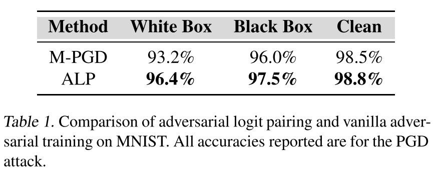
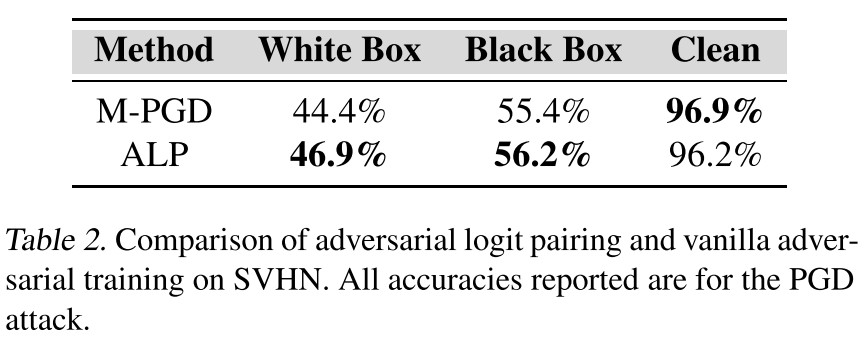
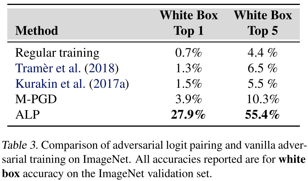
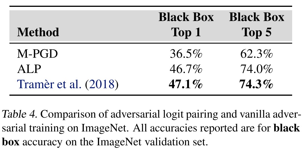
They also evaluate the proposed method on ImageNet.

Inspirations

This paper is very straightforward. The proposed Adversarial Logit Pair (ALP) is later verified and re-proposed in TRADES in a slightly different form with more theoretical supplements.

It's also very weird that Clean Logit Pair should increase robustness. If the increased robustness is caused by reducing the norm of logits, then it should be one of gradient masking intuitively.

Adversarial training for free - NIPS 2019

Code: https://github.com/ashafahi/free_adv_train

Ali Shafahi, Mahyar Najibi, Amin Ghiasi, Zheng Xu, John Dickerson, Christoph Studer, Larry S. Davis, Gavin Taylor, Tom Goldstein. Adversarial Training for Free! arXiv:1904.12843v2

The idea is to fasten the time-consuming adversarial training.

Free adversarial training

K-PGD adversarial training [Madry et al., 2017] is generally slow. For example, the 7-PGD training of a WideResNet [Zagoruyko and Komodakis, 2016] on CIFAR-10 in Madry et al. [2017] takes about four days on a Titan X GPU.

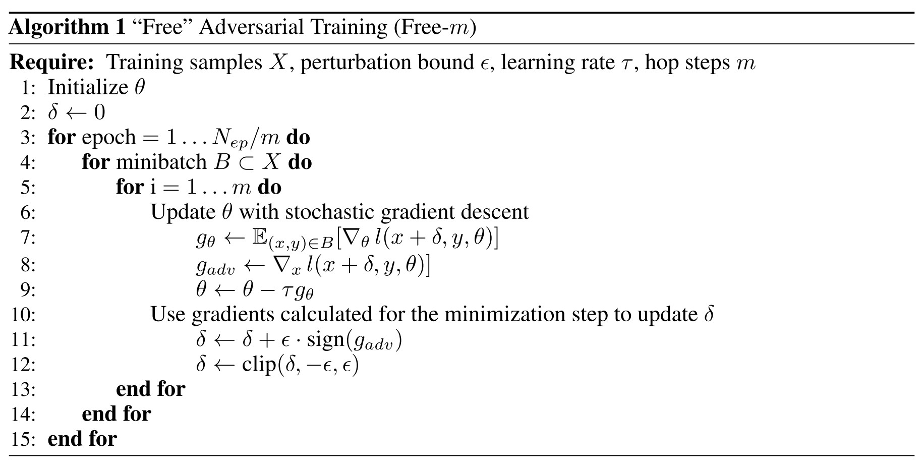
Our free adversarial training algorithm (alg. 1) computes the ascent step by re-using the backward pass needed for the descent step.

The original adversarial training launches $K$ steps of PGD to generate a batch of adversarial examples and then train the model, instead of which, they launches $1$ steps of PGD for the same batch and train model for $m$ times

Performance

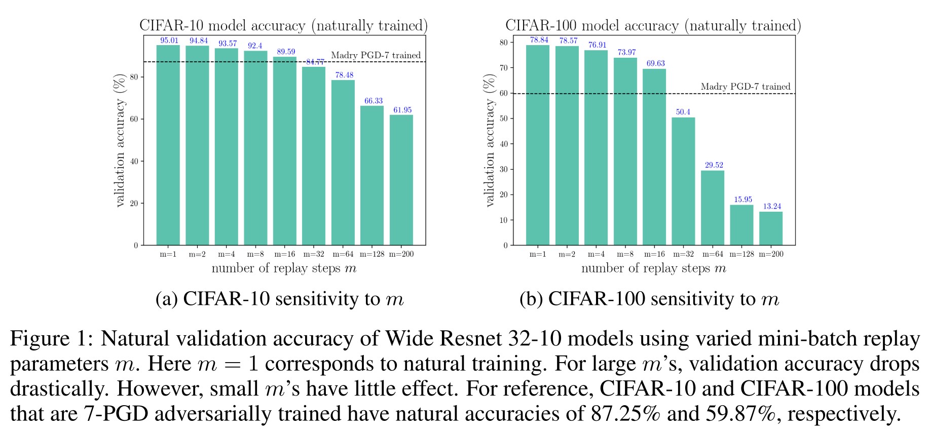
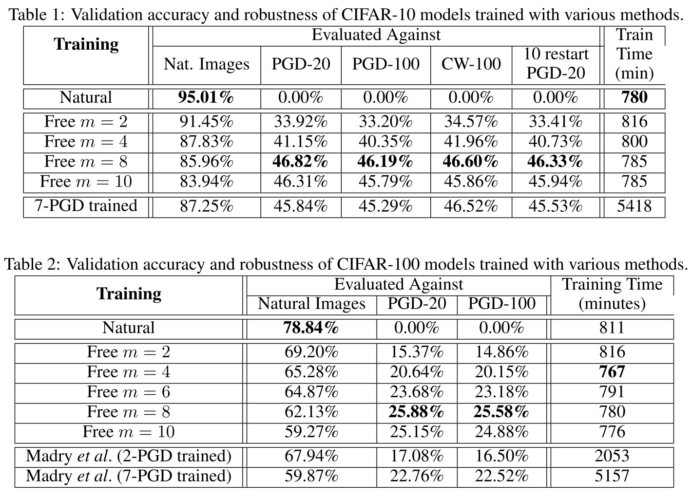
As shown above, the repeated training on the same batches compromises some accuracy and the robustness achieved with Free-m is comparable with that of adversarial training.

YOPO - NIPS 2019

Code: https://github.com/a1600012888/YOPO-You-Only-Propagate-Once

Paper: http://papers.nips.cc/paper/8316-you-only-propagate-once-accelerating-adversarial-training-via-maximal-principle

Dinghuai Zhang, Tianyuan Zhang, Yiping Lu, Zhanxing Zhu, Bin Dong. You Only Propagate Once: Accelerating Adversarial Training via Maximal Principle. NIPS 2019.

The idea is to accelerate adversarial training by eliminating the propagation rounds.

Through analyzing the Pontryagin’s Maximum Principle (PMP) of the problem, we observe that the adversary update is only coupled with the parameters of the first layer of the network.

Numerical experiments demonstrate that YOPO can achieve comparable defense accuracy with approximately 1/5 ∼ 1/4 GPU time of the projected gradient descent (PGD) algorithm.

The math is out of my reach.

UAT (Unsupervised Adversarial Training) - NIPS 2019

Code: https://github.com/deepmind/deepmind-research/tree/master/unsupervised_adversarial_training

Jonathan Uesato, Jean-Baptiste Alayrac, Po-Sen Huang, Robert Stanforth, Alhussein Fawzi, Pushmeet Kohli. Are Labels Required for Improving Adversarial Robustness?. NIPS 2019. arXiv:1905.13725

Given the discovery that adversarial training requires more data, which is generally not the case in real world, they explore the use of unlabeled data in adversarial training and find that it's a competitive alternative for adversarial training, compared to labeled data.

Our central hypothesis is that additional unlabeled examples may suffice for adversarial robustness.

• First, adversarial robustness depends on the smoothness of the classifier around natural images, which can be estimated from unlabeled data.
• Second, only a relatively small amount of labeled data is needed for standard generalization.

Setting

The classification problem considered here is to learn a predictor to map data into label, i.e.

They also assume access to a labeled training set

And an unlabeled training set

For standard classification, the objective is minimizing the natural risk, i.e.

For adversarial training, the primary objective is minimizing adversarial risk, i.e.

But since the inner optimization is intractable, the prevailing objective is a surrogate adversarial risk

Unsupervised adversarial training

Consider the decomposition of adversarial risk, i.e.

Just like the decomposition in TRADES.

The second loss, referred as smoothness loss, has no dependence on labels, thus possible to be tuned unsupervised.

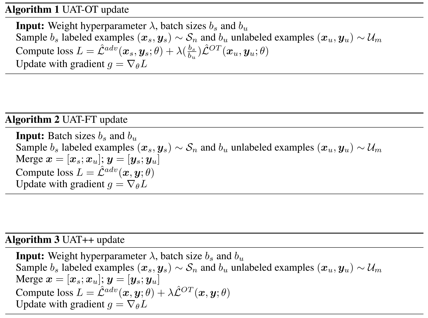
• UAT-OT (UAT with Online Targets)

  It directly minimizes a differentiable surrogate of the smoothness loss on the unlabeled data, i.e.

  $$\mathcal{L}_{\text {unsup }}^{O T}(\theta)=\underset{x \sim P(X)}{\mathbb{E}} \sup _{x^{\prime} \in \mathcal{N}_{\epsilon}(x)} \mathcal{D}\left(p_{\hat{\theta}}(. \mid x), p_{\theta}\left(. \mid x^{\prime}\right)\right)$$

  In which, $\mathcal{D}$ is the Kullback-Leiber divergence, and $\hat{\theta}$ refers to a fixed copy of parameters.

• UAT-FT (UAT with Fixed Targets)

  It first trains a standard classifier on the supervised set $\mathcal{S}_n$, then uses this classifier to generate pseudo labels for unlabeled data $\mathcal{U}_m$ such that one can employ standard adversarial training, i.e.

  $$\mathcal{L}_{\text {unsup }}^{F T}(\theta)=\underset{x \sim P(X)}{\mathbb{E}} \sup _{x^{\prime} \in \mathcal{N}_{\epsilon}(x)} \operatorname{xent}\left(\hat{y}(x), p_{\theta}\left(. \mid x^{\prime}\right)\right)$$

  In which, $xent$ refers to cross-entropy loss and $\hat{y}(x)$ is a pseudo-label obtained.

The overall training is thus a combination of supervised training and unsupervised training.

Experiments

To study the effect of unlabeled data, we randomly split the existing training set into a small supervised set $\mathcal{S}_n$ and use the remaining $N-n$ training examples as a source of unlabeled data.

We compare to the supervised oracle, which represents the best possible performance, where the model is provided the ground-truth label even for samples from $\mathcal{U}_m$.

For all experiments, we use variants of wide residual networks (WRNs) [52]. In Section 4.1, we use a WRN of width 2 and depth 28 for SVHN and a WRN of width 8 and depth 28 for CIFAR-10.

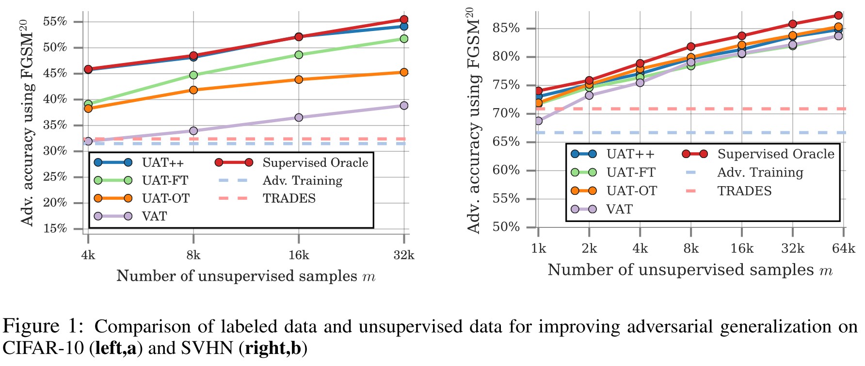
Empirically, we observe that UAT++, which combines the two approaches, outperforms either individually.

We demonstrate that, leveraging large amounts of unlabeled examples, UAT++ achieves similar adversarial robustness to supervised oracle, which uses label information.

They also observe that UAT is more robust to the label corruption to some extent.

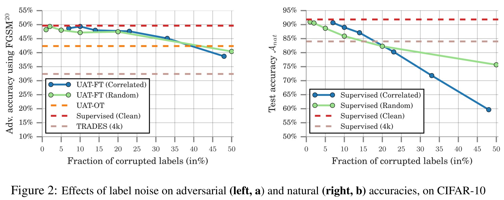
UAT shows significant robustness to label noise, achieving an 8.0% improvement over the baseline even with nearly 50% error in the base classifier.

They also investigate the effect of distributional shift in unlabeled data.

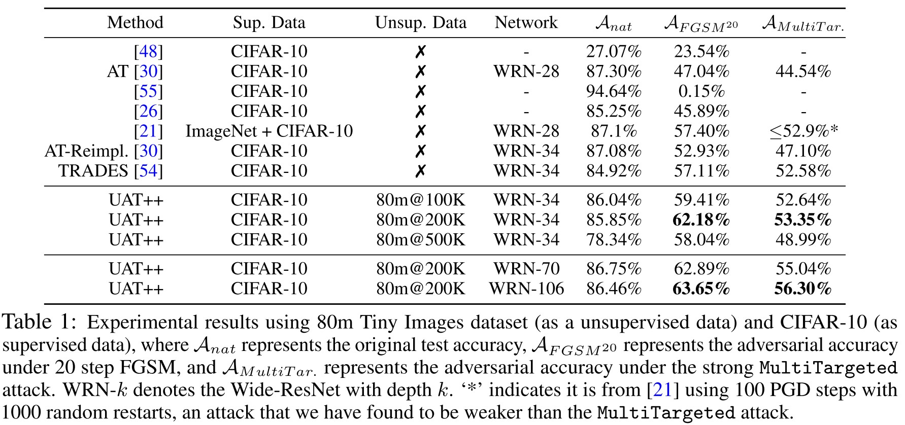
As shown in Table 1, despite the auto collected 80 Million Tiny Images is not always in distribution with those in CIFAR-10, UAT still increases the robustness and gives a new SOTA result.

Inspirations

With the same decomposition of adversarial loss as that in TRADES, they find that the smoothness loss has no dependence on labels, hence the possibility for it to be trained unsupervised.

Well, it also points a potential that since the classification loss is portable from the adversarial loss, it may be possible for two models to work together, one for classification and one for smoothness loss and adversarial robustness.

Attacks Which Do Not Kill Training Make Adversarial Learning Stronger - ICML 2020

Jingfeng Zhang, Xilie Xu, Bo Han, Gang Niu, Lizhen Cui, Masashi Sugiyama, Mohan Kankanhalli. Attacks Which Do Not Kill Training Make Adversarial Learning Stronger. ICML 2020. arXiv:2002.11242

We propose a novel formulation of friendly adversarial training (FAT): rather than employing most adversarial data maximizing the loss, we search for least adversarial data (i.e., friendly adversarial data) minimizing the loss, among the adversarial data that are confidently misclassified.

They propose the idea of friendly adversarial training and implement it by early stopping the PGD. (Fine, if you say so.)

Motivation

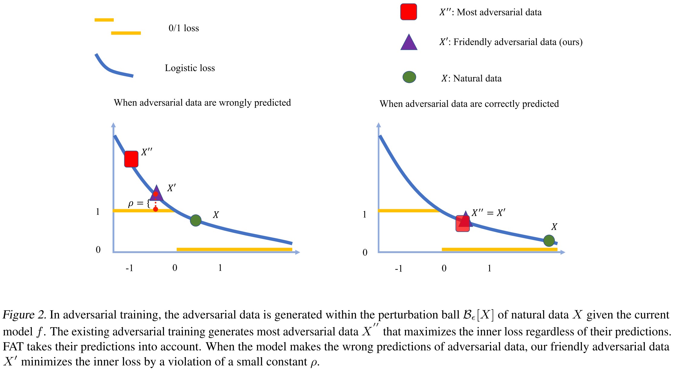
The standard adversarial training seeks to use the most adversarial example to train the network while the attackers only seek to find the least adversarial example (i.e. that can just fool the model), they intend to eliminate the inconsistency here.

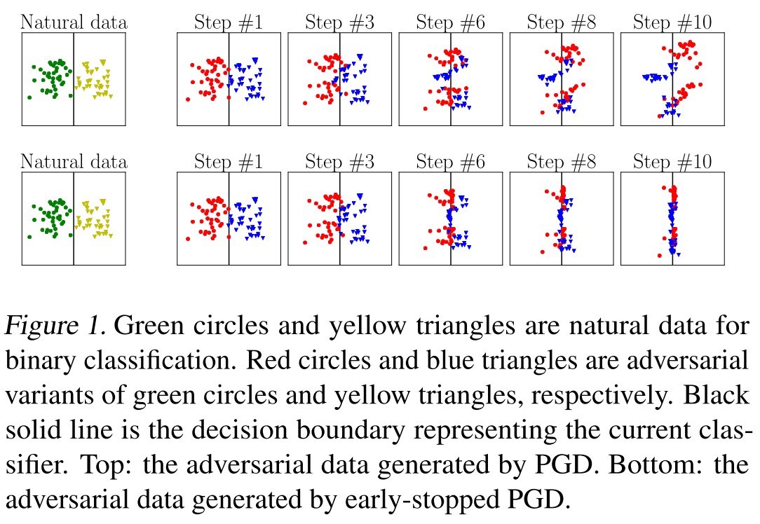
Besides, as shown in Figure 1, also as discovered in Robustness may be at Odds with Accuracy, a very strong adversary can cause crossover of adversarial examples, which makes the adversarial examples inappropriate for the classifier to learn a classification boundary (i.e. the boundary is severely corrupted), while as they proposed, using the least adversarial example will mitigate this problem.

Friendly adversarial training

The inner optimization in adversarial training ,i.e. the generation of adversarial example is proposed to use

The adversarial example is sought inside a $l_{\infty}$-bounded ball, i.e.

They employ the adversarial risk defined in TRADES, i.e.

And give an upper bound of their own

Theorem 1 For any classifier $f$, any non-negative surrogate loss function $\ell$ which upper bounds the 0/1 loss, and any probability distribution $\mathcal{D}$, there is

where

If the perturbed example is not misclassified, then continuing perturbing by maximizing the classification loss;otherwise, find the least adversarial example in a $\rho$-band of the boundary.

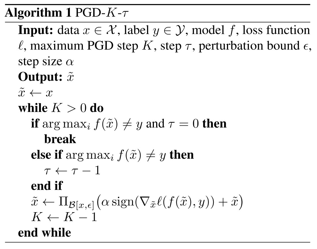
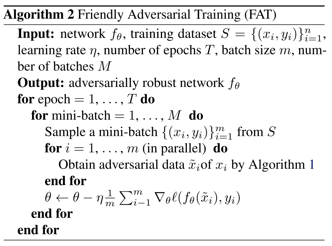
Algorithm

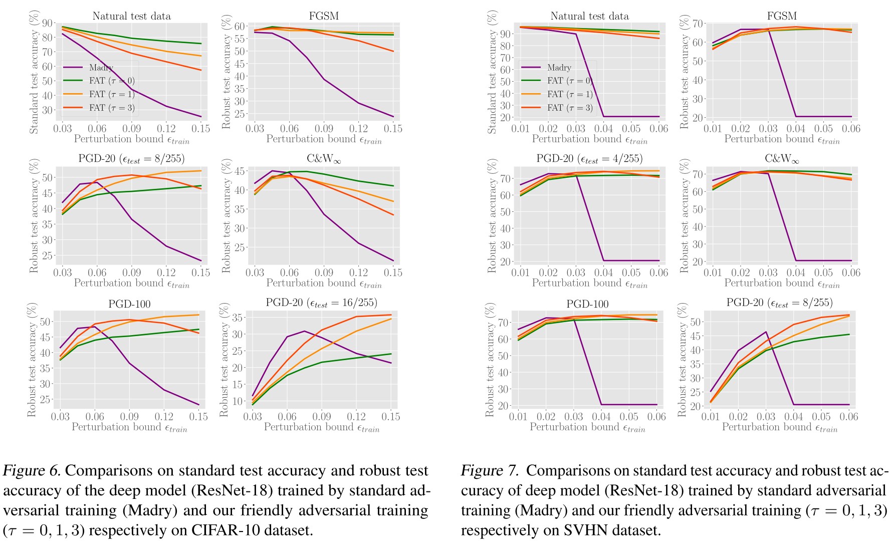
Experiments

Inspirations

This is an expected work given the paper Robustness may be at Odds with Accuracy, which points out that a very strong adversary can flip the distribution of data, thus making the learning of classifier completely wrong headed.

Nevertheless, it's still very nice to see that it do work.

Smooth adversarial training - 2020

Cihang Xie, Mingxing Tan, Boqing Gong, Alan Yuille, Quoc V. Le. Smooth Adversarial Training. arXiv:2006.14536

They find out that the sharp gradient of ReLU tampers the adversarial training process and designed a smooth surrogate to replace ReLU for better robustness gained by adversarial training.

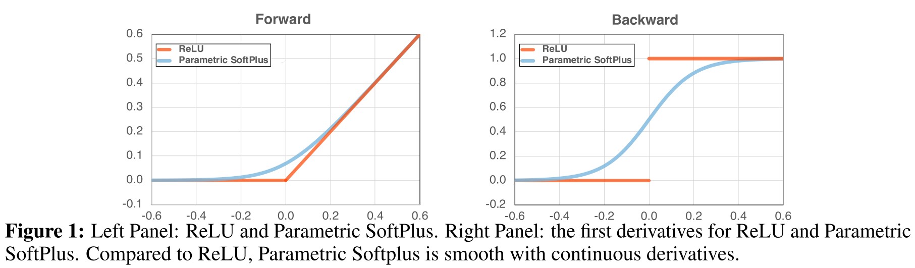
Existing works suggest that, to further improve adversarial robustness, we need to either sacrifice accuracy on clean inputs, or incur additional computational cost. This phenomenon is generally referred to as the no free lunch in adversarial robustness.

How gradient quality affects adversarial training

Adversarial training consists of a two optimization problems:

The inner maximization step attempts to craft adversarial examples and the outer minimization step attempts to adjust the parameters according to both the clean and adversarial examples.

They conjecture that since the adversarial training requires the computation of gradients both on the input and the parameters, the non-smooth nature will hurt the training process.

It sounds not that convincing, since the activation is applied both to the input and parameter, i.e. when backpropagate the gradients either to the parameter or to the input, the non-smoothness of activation affects both process.

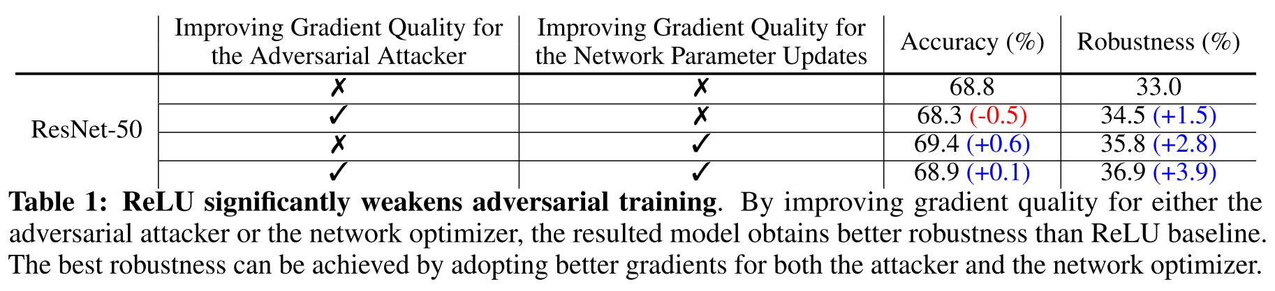
To check the influence of smoothness of gradients, they replace the ReLU in the backpropogation of adversarial training's inner round with a smooth substitute. In inference and adversarial training's outer round, the ReLU activation is unchanged.

As shown in the table 1, it appears that the adversarial training is enhanced by the better gradient quality.

They also tested some basic training enhancements:

• More attack iterations

  By increasing the attacker’s cost by 2×, PGD-2 improves the ReLU baseline by 0.6% for robustness while losing 0.1% for accuracy. This result suggests we can remedy ReLU’s gradient issue in the inner step of adversarial training if more computations are given.

• Training longer

  Longer training gains 2.6% for accuracy but loses 1.8% for robustness. On the contrary, applying better gradients for optimizing networks in the previous section improves both robustness and accuracy. This discouraging result suggests that training longer cannot fix the issues in the outer step of adversarial training caused by ReLU’s poor gradient.

Smooth adversarial training

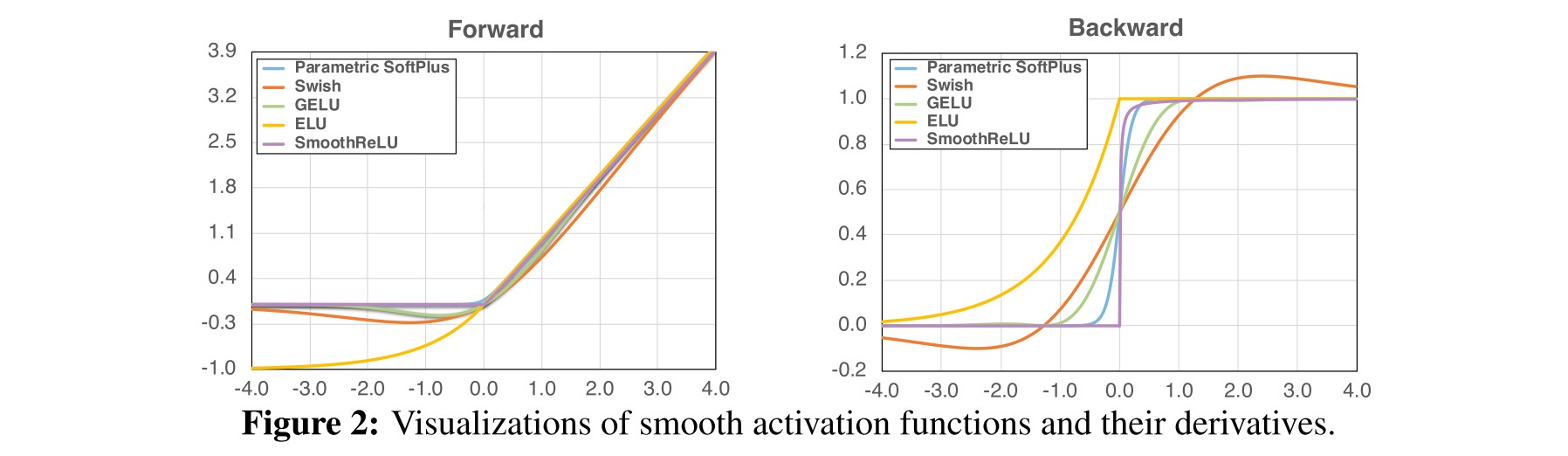
They further explored a series approximate of ReLU, including:

• Softplus

  $$f(x)=\frac{1}{\alpha}\mathop{log}(1+\mathop{exp}(\alpha x))$$

• Swish

  $$f(x)=x\cdot \mathop{sigmoid}(x)$$

• Gaussian Error Linear Unit

  $$f(x)=x\cdot\Phi(x)$$

  In which, $\Phi(x)$ is the cumulative distribution function of the standard normal distribution.

• Exponential Linear Unit (ELU)

  $$\mathop{ELU}(x,\alpha)=\begin{cases} x &\text{if}\ x\ge 0,\\ \alpha(\mathop{exp}(x)-1)&\text{otherwise} \end{cases}$$

And they propose their smooth ReLU activation, defined as:

It's derivative is:

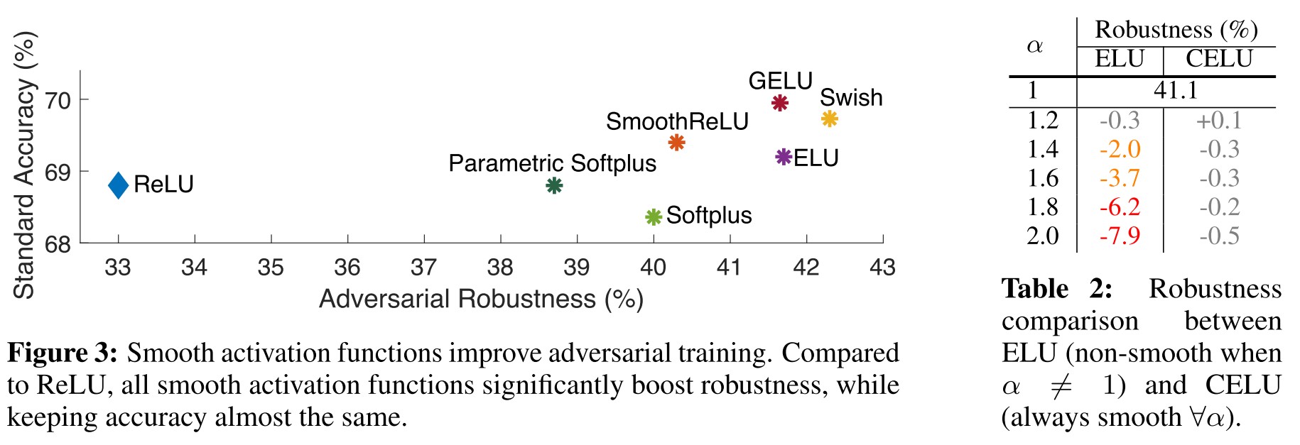
We observe SmoothReLU substantially outperforms ReLU by 7.3% for robustness (from 33.0% to 40.3%), and by 0.6% for accuracy (from 68.8% to 69.4%)

How network scaling-up affects robustness

Tan et al. [40] suggest that, all three scaling-up factors, i.e., depth, width and image resolutions, are important to further improve ResNet performance.

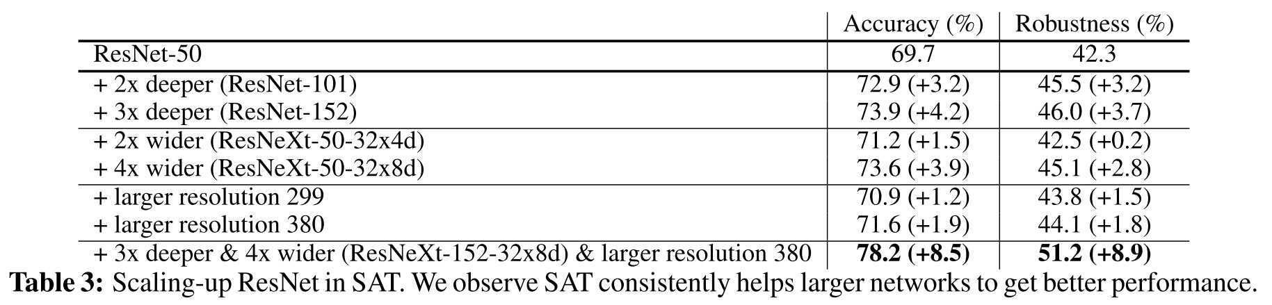
We confirm that both deeper or wider networks consistently outperform the baseline network in SAT.

We conjecture this improvement is possible because a larger image resolution (1) enables attackers to create stronger adversarial examples [10]; and (2) increases network capacity [40], therefore benefits SAT overall.

All these robustness performances are lower than the robustness (42.3%) achieved by the ResNet-50 baseline in SAT (first row of Table 3). In other words, scaling up networks seems less effective than replacing ReLU with smooth activation functions.

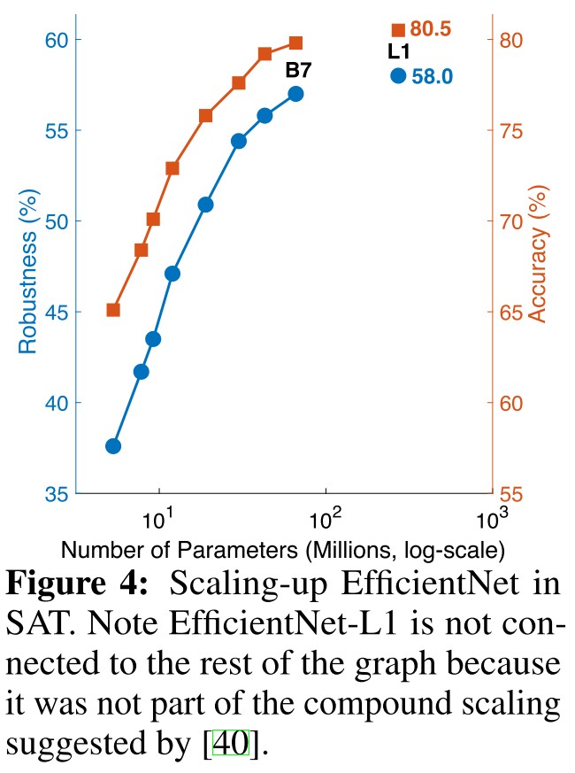
EfficientNet [40], which uses neural architecture search to automatically discover the optimal factors for network scaling, provides a strong family of models for image recognition.

Adversarial training +

TRADES - ICML 2019

Code: https://github.com/yaodongyu/TRADES

Hongyang Zhang, Yaodong Yu, Jiantao Jiao, Eric P. Xing, Laurent El Ghaoui, Michael I. Jordan. Theoretically Principled Trade-off between Robustness and Accuracy. ICML 2019. arXiv:1901.08573

They decompose the prediction error of adversarial examples into the sum of a classification error and a boundary error and provide an upper bound. Based on the theory, they design a defense method named as TRADES.

Robust error and boundary error

Given a set of instances $x_1,\dots,x_n\in\cal{X}$ and labels $y_1,\dots,y_n\in\{-1,+1\}$, the data is assumed to be sampled from an unknown distribution $(\bold{X},Y)\sim\cal{D}$. The classification is made by $sign(f(x))$, i.e. the sign of a score function $f:\cal{X}\to\R$.

The robust (classification) error of a score function $f:\mathcal{X}\to\R$ is defined as

In which, $\Bbb{B}(\bold{X},\epsilon)$ is a neighborhood of $\bold{X}$, i.e.

In human words, the robustness is defined as the expectation of the probability that an adversarial example exists in an $\epsilon$ neighborhood over all instances.

The natural (classification) error is defined as

In contrast, the classification error is actual the expectation of the probability that an example is misclassified over all instances.

It's obvious that

The same but looser conclusion as the Theorem 2 in "Adversarial Vulnerability in any Classifier".

They introduce a third error, i.e. the boundary error, defined as

In which, $DB(f)$ denotes the decision boundary of $f$, i.e.

and $\Bbb{B}(DB(f),\epsilon)$ is therefore the neighborhood of the decision boundary, i.e.

The boundary error is defined as the expectation that all points in the $\epsilon$-neighborhood of the boundary are correctly classified .(? I think there is a typo.)

The robustness error can be decomposed as

Relating 0-1 loss to surrogate loss

Minimizing the 0-1 loss is computational intractable, for which, a surrogate loss is introduced, i.e.

They assume that $\phi$ is classification-calibrated.

Formally, for $\eta\in[0,1]$, define the conditional $\phi$-risk by

$$H(\eta):=\inf_{\alpha\in\R}C_{\eta}(\alpha):=\inf_{\alpha\in\R}(\eta\phi(\alpha)+(1-\eta)\phi(-\alpha))$$

define $H^{-}(\eta):=\inf_{\alpha(2\eta-1)\le 0}C_{\eta}(\alpha)$. The classification-calibrated condition requires that imposing the constraint that $\alpha$ has an inconsistent sign with the Bayes decision rule $sign(2\eta-1)$ leads to a strictly larger $\phi$-risk:

Assumption 1 (Classification-Calibrated Loss) We assume that the surrogate loss $\phi$ is classification-calibrated, meaning that for any $\eta\neq 1/2$, $H^{-1}(\eta)>H(\eta)$.

Theorem 3.1 Let $\mathcal{R}_{\phi}(f):=\Bbb{E}_{\phi}(f(\bold{X})Y)$ and $\mathcal{R}_{\phi}^*:=\min_f\mathcal{R}_{\phi}(f).$ Under Assumption 1, for any non-negative loss function $\phi$ such that $\phi(0)\ge 1$, any measurable $f:\mathcal{X}\to\R$, any probability distribution on $\mathcal{X}\times\{-1,+1\}$, and any $\lambda>0$, we have

Theorem 3.2 Suppose that $|\mathcal{X}|\ge 2$. Under Assumption 1, for any non-negative loss function $\phi$ such that $\phi(x)\to 0$ as $x\to+\infty$, any $\xi>0$, and any $\theta\in[0,1]$, there exists a probability distribution on $\mathcal{X}\in\{-1,+1\}$, a function $f:\R^d\to\R$, and a regularization parameter $\lambda>0$ such that $\mathcal{R}_{rob}(f)-\mathcal{R}^*_{nat}=0$ and

Adversarial training by TRADES

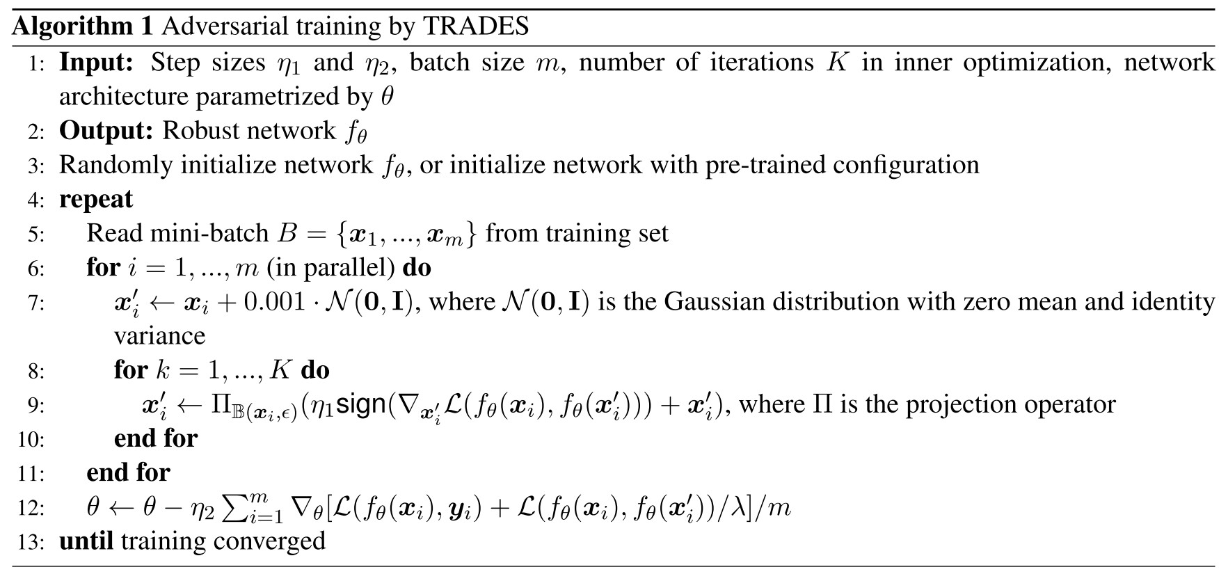
In order to minimize $\mathcal{R}_{rob}(f)-\mathcal{R}^*_{nat}$, the theorems suggests minimizing

This is exactly the purpose of adversarial training in a binary classification problem, but the problem is slightly modified, the adversarial examples are not generated to fool the labels but to fool the current predictions.

Extended to multi-class form, it becomes

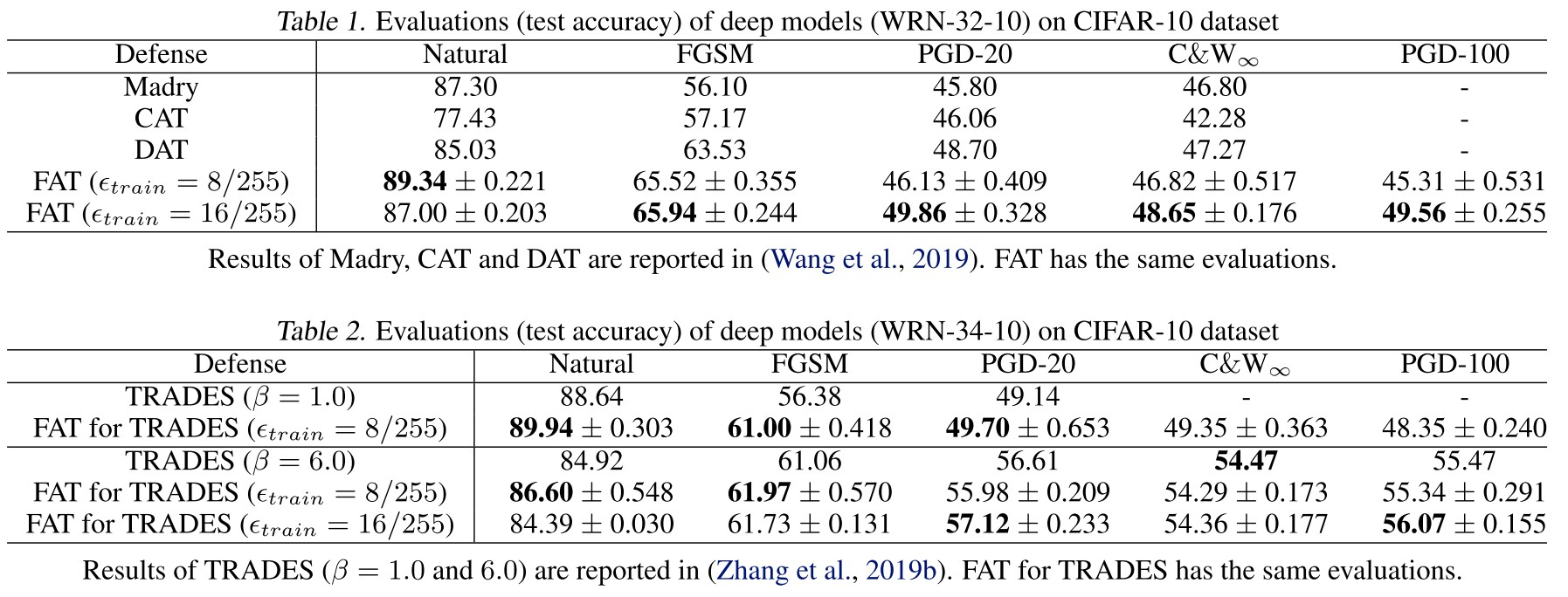
Experiments

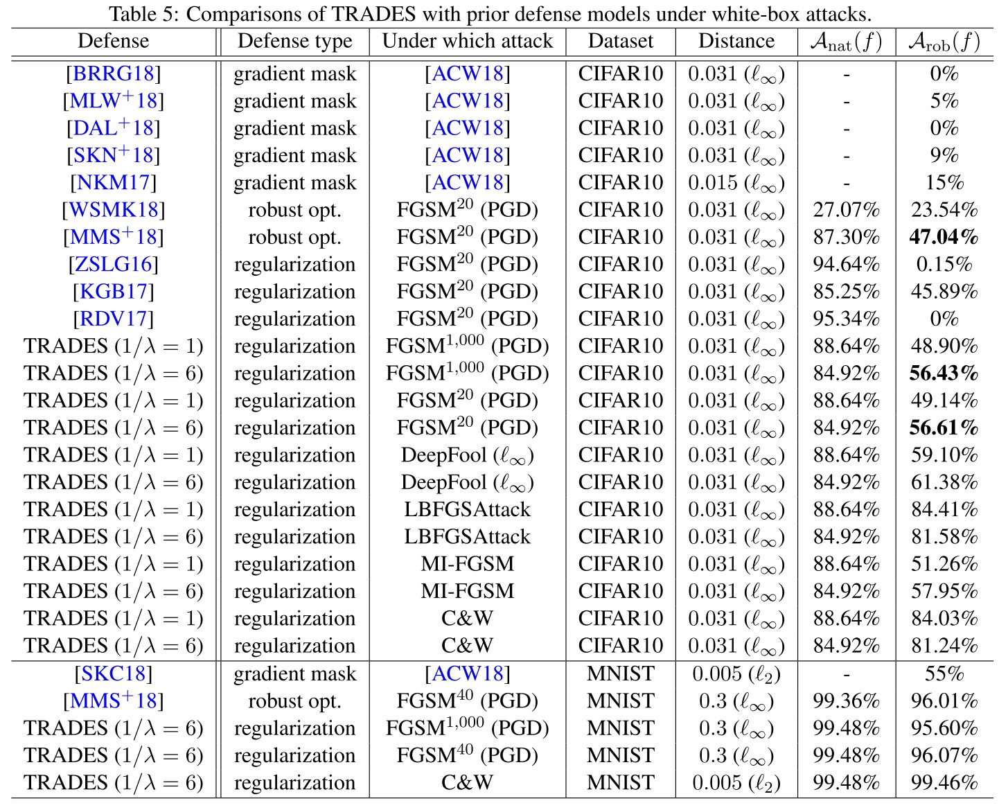
The notations used in Table 5:

• $\cal{A}_{nat}(f)$ - natural accuracy
• $\cal{A}_{rob}(f)$ - robust accuracy

Feature denoising - CVPR 2019

Code: https://github.com/facebookresearch/ImageNet-Adversarial-Training

Cihang Xie, Yuxin Wu, Laurens van der Maaten, Alan Yuille, Kaiming He. Feature Denoising for Improving Adversarial Robustness. CVPR 2019. arXiv:1812.03411

They discover that adversarial example results a more noisy feature map in the network, based on which, they propose feature denoising, combined with adversarial training to produce a more robust model.

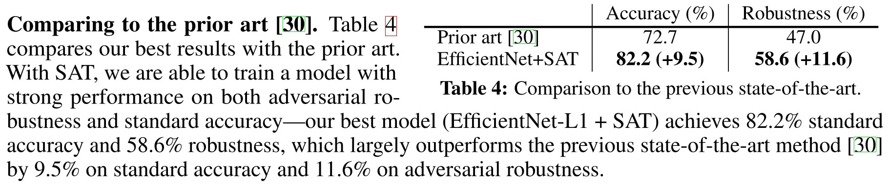
When combined with adversarial training, our feature denoising networks substantially improve the state-of-the-art in adversarial robustness in both white-box and black-box attack settings.

Feature noise

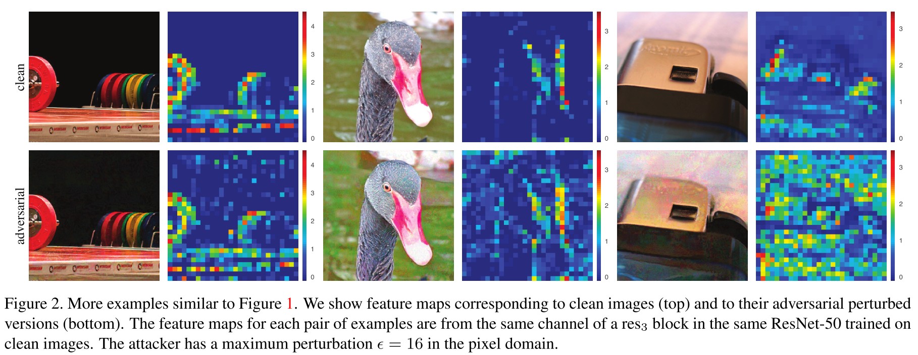
As shown in Figure 2, the adversarial perturbations incites hallucinated activations in the feature.

We found it is nontrivial to compare feature noise levels between different models, in particular, when the network architecture and/or training methods (standard or adversarial) change.

These feature noise is easy to qualitatively measure, but difficult to quantitatively measure.

Denoising block

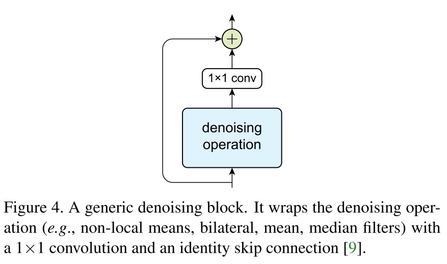
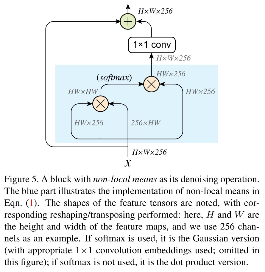
The generic framework of a denoising block is shown in Figure 4, the residual connection and $1\times 1$ convolution are mainly for feature combination while the denoising operation is the key part.

Using the non-local like operation, in Figure 5 there is their instantiation of denoising block.

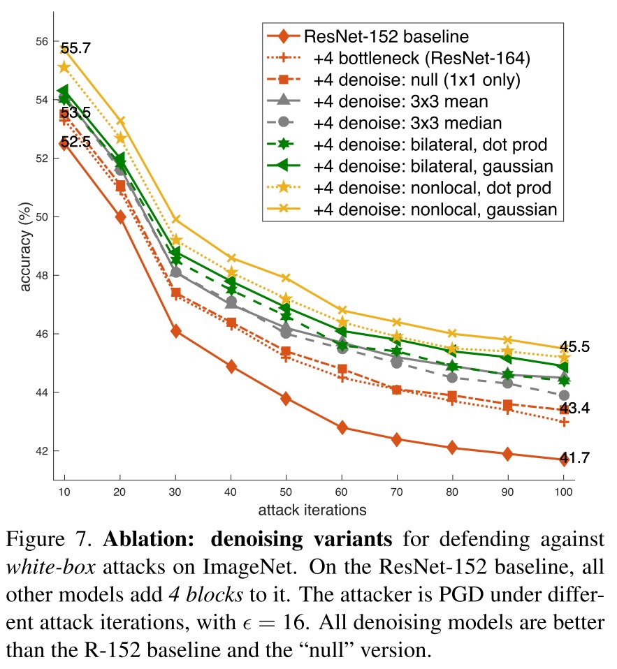
They explore the following denoise operations:

• Non-local means

  It computes a denoised feature map $y$ of an input feature map $x$ by taking a weighted mean of features in all spatial locations $\mathcal{L}$, i.e.

  $$y_i=\frac{1}{\mathcal{C}(x)}\sum_{\forall j\in \mathcal{L}}f(x_i,x_j)\cdot x_j$$

  In which, $f(x_i,x_j)$ is a feature-dependent weighting function and $\mathcal{C}(x)$ is a normalization function.

  The following weighting functions are considered

  • Gaussian (softmax) sets

    With two embedded versions of $x$, i.e. $\theta(x)$ and $\phi(x)$:

    $$f(x_i,x_j)=e^{\frac{1}{\sqrt{d}}\theta(x_i)^{\top}\phi(x_j)},\\ \mathcal{C}=\sum_{\forall j\in\mathcal{L}}f(x_i,x_j)$$

  • Dot product sets

    $$f(x_i,x_j)=x_i^\top x_j,\\ \mathcal{C}(x)=N$$

    The dotproduct version provides a denoising operation with no extra parameters (blue box in Figure 5).

• Bilateral filter

  Turn the "non-local" into "local", it becomes the bilateral filter popular for edge-preserving denoising, i.e.

  $$y_i=\frac{1}{\mathcal{C}(x)}\sum_{\forall j\in\Omega(i)}f(x_i,x_j)\cdot x_j$$

  In which, $\Omega(i)$ is a local region around pixel $i$ (e.g. $3\times 3$ patch).

• Mean filter

  However, somewhat surprisingly, experiments show that denoising blocks using mean filters as the denoising operation can still improve adversarial robustness.

• Median filter

  $$y_i=\text{median}\{\forall j\in\Omega(i):x_j\}$$

  We find experimentally that using median filters as a denoising operation can also improve adversarial robustness.

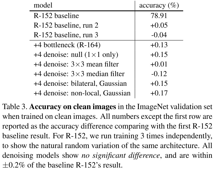
Experiments

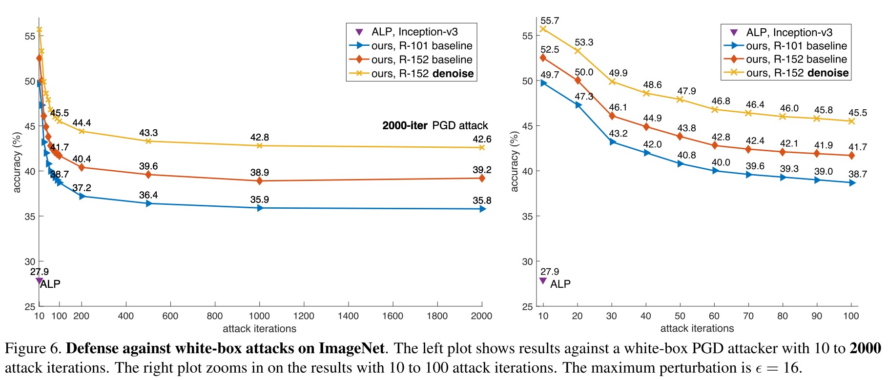
There is a consistent performance improvement introduced by the denoising blocks. Under the 10-iteration PGD attack, it improves the accuracy of ResNet-152 baseline by 3.2% from 52.5% to 55.7% (Figure 6, right).

Inspirations

It's surely inspiring that the feature maps are noisy in the face of adversarial examples, but it's also disappointing that by denoising feature maps, one still requires adversarial training to achieve satisfactory robustness. Nevertheless, the robustness gain is fairly good.

Is it possible to denoise the feature somehow and achieve robustness without the computational expensive adversarial training?

Fast adversarial training

Fast is better than free - ICLR 2020

Paper: https://openreview.net/forum?id=BJx040EFvH¬eId=BJx040EFvH

Eric Wong, Leslie Rice, and J. Zico Kolter. Fast is better than free: Revisiting adversarial training. ICLR, 2020

Most of the contributions of this work is revisited and covered in Understanding and Improving Fast Adversarial Training, and some of the conclusions are even challenged, therefore the note for this paper will be relatively short.

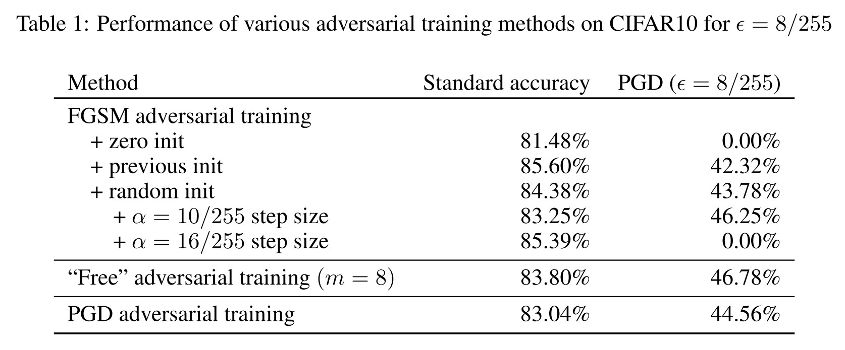
They find that FGSM-based adversarial training with random initialization is as effective as PGD-based adversarial training.

Motivation

A property of free adversarial training is that the perturbation from the previous iteration is used as the initial starting point for the next iteration.

We hypothesize that the main benefit comes from simply starting from a non-zero initial perturbation.

Crucially, we find that starting from a non-zero initial perturbation is the primary driver for success, regardless of the actual initialization.

This is actually quite reasonable, since starting from various random initialization enriches the diversity of generated adversarial examples.

They find that a large step size results in catastrophic overfitting

However, we also found that forcing the resulting perturbation to lie on the boundary with a step size of α = 2 resulted in catastrophic overfitting.

And the computational complex for FGSM adversarial training and free adversarial training are

• Free adversarial training uses a single backwards pass to compute gradients for both the perturbation and the model weights while repeating the same minibatch $m$ times in a row, called “minibatch replay”.
• The computational complexity for an epoch of FGSM adversarial training is not truly free and is equivalent to two epochs of standard training.

FGSM RS

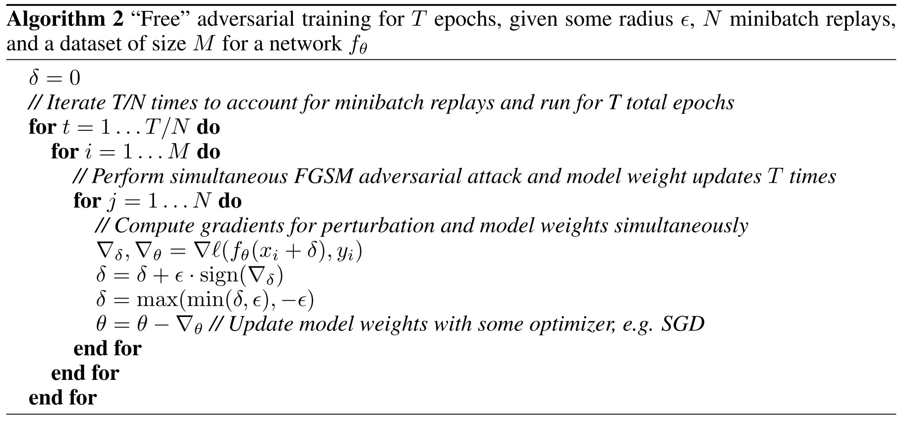
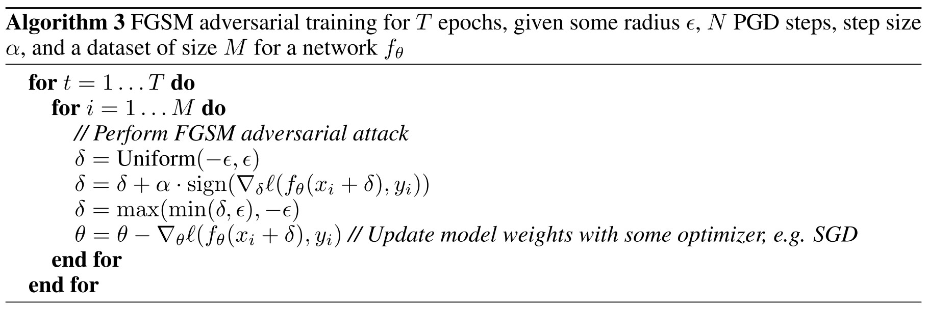
In Algorithm 3 there is the proposed FGSM adversarial training with random initialization (FGSM RS), as shown in table, in each epoch, the number of gradient computations for free adversarial training (Algorithm 2) is proportional to $O(MN)$, while that for FGSM RS is $O(M)$.

Understanding and Improving Fast Adversarial Training - NIPS 2020

Code: https://github.com/tml-epfl/understanding-fast-adv-training

Paper: https://infoscience.epfl.ch/record/278914

Maksym Andriushchenko, Nicolas Flammarion. Understanding and Improving Fast Adversarial Training. NIPS 2020.

We show that adding a random step to FGSM, as proposed in [47], does not prevent catastrophic overfitting, and that randomness is not important per se — its main role being simply to reduce the magnitude of the perturbation.

They try to improve FGSM-based adversarial training. Based on the recent discovery that FGSM-based adversarial training suffers from catastrophic overfitting, they intend to probe the following question:

When and why does fast adversarial training with FGSM lead to robust models?

Problem

Denote $\ell(x,y;\theta)$ as the loss of a ReLU-network (?) parameterized by $\theta\in \R^m$ on the example $(x,y)\sim D$, where $D$ is the data generating distribution. Adversarial training aims to solve the following optimization problem:

Here, they focus on the $l_{\infty}$ threat model, i.e. $\Delta=\{\delta\in \R^d,||\delta||_{\infty}\le\varepsilon\}$.

The inner optimization problem has to be solved independently due to the fact that each subproblem depends on the particular example pairs $(x,y)$, hence an inherent trade-off appears between computational efficiency and solving accuracy.

FGSM is proposed to solve the problem fast but not accurate, i.e.

And the resulted adversarial example is the projection of $x+\delta_{FGSM}$ on $[0,1]^d$ to ensure its validity.

A closer look at the evolution of the robustness during FGSM AT reveals that using FGSM can lead to a model with some degree of robustness but only until a point where the robustness suddenly drops. (namely catastrophic overfitting)

Wong et al. propose to initialize FGSM from a random starting point to mitigate the catastrophic overfitting, i.e.

Along the same lines, [43] observe that using dropout on all layers (including convolutional) also helps to stabilize FGSM AT.

An alternative solution is to interpolate between FGSM and PGD AT.

Investigation of FGSM-RS

FGSM with random step does not resolve catastrophic overfitting

It only works when $\varepsilon$ is small, the problem still exists for larger $\varepsilon$.

Previous explanation: randomness diversifies the threat model

We conclude that diversity of adversarial examples is not crucial here. What makes the difference is rather having an iterative instead of a single-step procedure to find a corner of the $l_{\infty}$-ball that sufficiently maximizes the loss.

New explanation: a random step improves the linear approximation quality

Using a random step in FGSM is guaranteed to decrease the expected magnitude of the perturbation.

Lemma 1. (Effect of the random step) Let $\eta\sim\mathcal{U}([-\varepsilon,\varepsilon]^d)$ be a random starting point, and $\alpha\in[0,2\varepsilon]$ be the step size of FGSM-RS, then

Since $||\delta_{FGSM}||_2=\sqrt{d}\varepsilon$, therefore FGSM-RS reduces the magnitude of step.

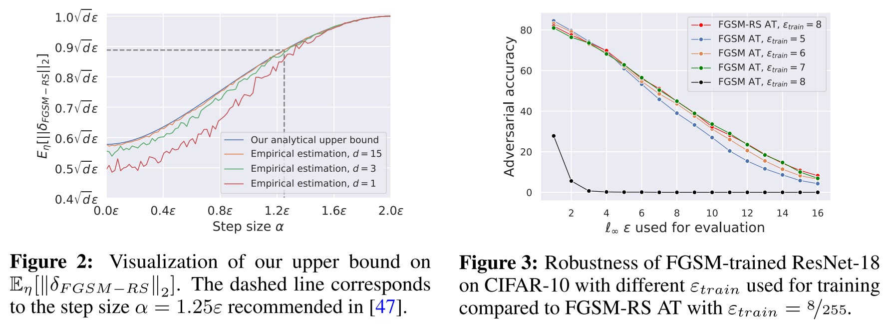
The key observation here is that among all possible perturbations of $l_{\infty}$-norm $\varepsilon$, perturbations with a smaller $l_2$-norm benefit from a better linear approximation. (A smaller $||\delta||_2$ implies a smaller linear approximation error.​)

Successful FGSM AT does not require randomness

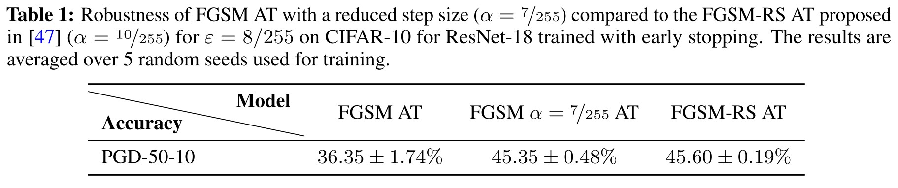
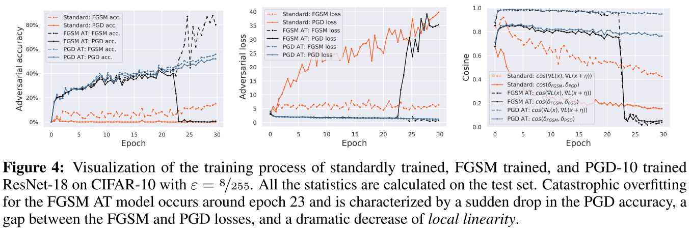
As shown in Table 1, just reducing the step size of standard FGSM can achieve comparable robustness accuracy with FGSM-RS.

Gradient alignment

The FGSM attack is obtained as a closed-form solution to the following problem

The FGSM is guaranteed to find the optimal adversarial perturbation if $\nabla_x\ell(x,y;\theta)$ is constantly inside the $l_{\infty}$-ball around the input $x$, i.e. the loss function is locally linear.

They then propose a local linearity metric as gradient alignment, i.e.

It's a little confusing, I think they mean the cosine similarity metric.

With the local linearity metric, it's not possible to check what happened in FGSM adversarial training.

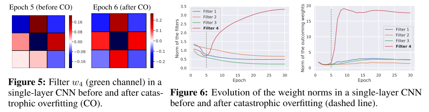
As shown in Figure 4, catastrophic in FGSM AT occurs around epoch 23, along with two changes

1. There is a sudden drop in the PGD accuracy from 40.1% to 0.0%, along with an abrupt jump of the FGSM accuracy from 43.5% to 86.7%.
2. Concurrently, after catastrophic overfitting, the gradient alignment of the FGSM model experiences a phase transition and drops significantly from 0.95 to 0.05 within an epoch of training, i.e. the input gradients become nearly orthogonal inside the $l_{\infty}$-ball

This echoes the observation made in [26] that SGD on the standard loss of a neural network learns models of increasing complexity.

They further empirically observe that even a single convolutional filter can cause catastrophic overfitting.

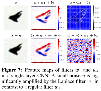
After the catastrophic overfitting (CO), one the filters goes virus and turned into a variant of the Laplace filter, which is known for amplifying high-frequency noise. Another cue is that the model starts training from highly aligned gradient.

A single-layer CNN is easy to handle. Let $Z\in\R^{p\times k}$ be the matrix of $k$ non-overlapping image patches extracted from the image $x=vec(Z)\in\R^d$ such that $z_j=z_j(x)\in\R^p$. The model prediction (with ReLU-activation) $f$ is parameterized by $(W,b,U,c)\in\R^{p\times m}\times\R^m\times\R^{m\times k}\times\R$, its prediction and gradient in input is

Lemma 2. (Gradient alignment at initialization) Let $z\sim\mathcal{U}([0,1]^p)$ be an image patch for $p\ge 2$, $\eta\sim\mathcal{U}([-\varepsilon,\varepsilon]^d)$ is a point inside the $l_{\infty}$-ball, the parameters of a single-layer CNN initialized i.i.d. as $w\sim\mathcal{N}(0,\sigma^{2}_{w}I_p)$ for every column of $W$, $u\sim\mathcal{N}(0,\sigma^2_{u}I_{m})$ for every column of $U$, $b:=0$, then the gradient alignment is lower bounded by

Thus, it appears to be a general phenomenon that the standard initialization scheme of neural network weights [15] ensures the initial success of FGSM training.

For deep networks, however, we could not identify particular filters responsible for catastrophic overfitting, thus we consider next a more general solution.

GradAlign regularizer for fast adversarial training

GradAlign

Based on the observations above, they propose a regularizer named as GradAlign. It's designed to maximize the gradient alignment between the gradients at point $x$ and at a randomly perturbed point $x+\eta$ inside the $l_{\infty}$-ball around $x$, i.e.

This regularizer only depends on the gradient direction.

Intuitively, this regularizer reforms the gradients for the FGSM to work better.

Experiments

We train these methods using PreAct ResNet-18 [16] with $l_{\infty}$-radii $\varepsilon\in\{1/255,\dots,16/255\}$ on CIFAR-10 for 30 epochs and $\varepsilon\in \{1/255,\dots,12/255\}$ on SVHN for 15 epochs. The only exception is AT for Free [34] which we train for 96 epochs on CIFAR-10, and 45 epochs on SVHN which was necessary to get comparable results to the other methods.

Also, we remark that training with GradAlign leads on average to a 3× slowdown on an NVIDA V100 GPU compared to FGSM training which is due to the use of double backpropagation (see [9] for a detailed analysis).

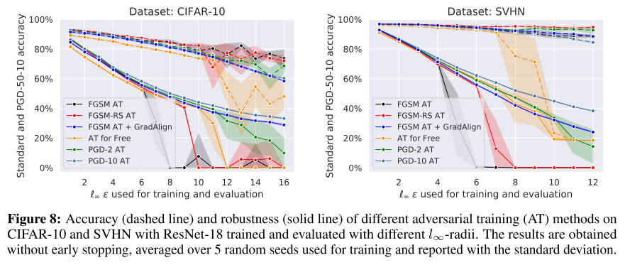
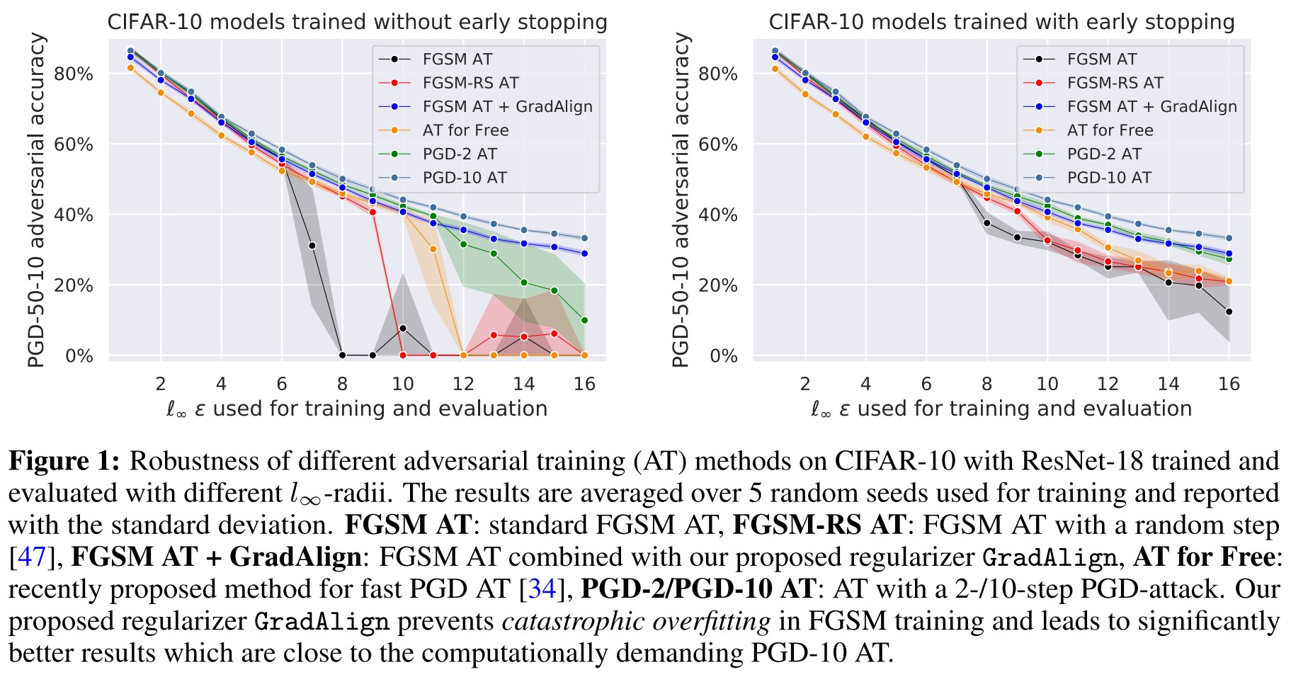
As shown in Figure 8, GradAlign mitigates the problem of catastrophic overfitting for FGSM adversarial training, and AT for free and PGD-2 is also appeared to face catastrophic overfitting with higher $\varepsilon$.

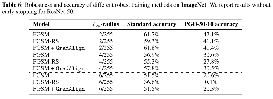
In ImagNet, they find that for small bounds, the catastrophic overfitting doesn't occur even in standard FGSM adversarial training and for $\varepsilon=6/255$, catastrophic overfitting occurs very early in training (around 3) (Why?).

We observed that training FGSM + GradAlign for more than 30 epochs also leads to slightly worse robustness on the test set (see Appendix D.4), thus suggesting that catastrophic and robust overfitting (proposed with a solution of early stopping) are two distinct phenomena that have to be addressed separately.

This discovery is unexpected, since intuitively robust overfitting should be the catastrophic overfitting in PGD adversarial training.

Inspiration

This paper is the scientific research in my dream !

They go from the phenomenon to the mechanism behind it, questioning the concurrent hypothesis and grounding their own explanation with solid theoretical and empirical results. They then evaluate their own hyothesis and verify that the misalignment of gradients is likely to be the reason for catastrophic overfitting in FGSM adversarial training. With the verified hypothesis, they then propose their own method, namely GradAlign to solve the problem.

They also leave a lot of potential future works to do

• Improve th GradAlign, since the original one they proposed is very basic
• Sort out the reason behind the different performances of FGSM-RS in ImageNet.
• Handle with the robust overfitting possibly with similar techniques in this paper.
• Delve into the phenomenon of gradient misalignment in fast adversarial training, I think there is more behind it.