Adversarial Defense by Regularization
By LI Haoyang 2020.11.6
Content
Adversarial Defense by RegularizationContentLipschitz RegularizationParseval Networks - ICML 2017Robustness in neural networksGeneralization with adversarial examplesLipschitz constant of neural networksParseval networksParseval trainingExperimentsInspirationsLinear RegularizationAdversarial robustness through local linearization - NIPS 2019Adversarial trainingLocal linearity measureLocal linear regularizer (LLR)ExperimentLogit RegularizationImproved Adversarial Robustness via Logit Regularization Methods - 2019Adversarial Logit Pairing and Logit RegularizationLabel SmoothingDecoupling Adversarial Logit PairingExperimentsInspirationsJacobian RegularizationJARN (Jacobian Regularization) - ICLR 2020Jacobian Adversarially Regularized NetworksTheoretical analysis of JARNExperimentsInspirations
Lipschitz Regularization
Parseval Networks - ICML 2017
Moustapha Cisse , Piotr Bojanowski, Edouard Grave, Yann Dauphin, Nicolas Usunier. Parseval Networks: Improving Robustness to Adversarial Examples. ICML 2017. arXiv:1704.08847
We introduce Parseval networks, a layerwise regularization method for reducing the network’s sensitivity to small perturbations by carefully controlling its global Lipschitz constant.
Our main idea is to control this norm by parameterizing the network with parseval tight frames (Kovaˇcevi´c & Chebira, 2008), a generalization of orthogonal matrices.
Robustness in neural networks
They consider a multiclass prediction setting.
The classifier is a function that maps data to its correct label , parameterized by weights :
The score is given to the input-class pair by a function , which is assumed to be a neural network, represented by a computation graph .
Each node takes values in and is a function of its children in the graph, with learnable parameters :
The learned function is the root of . The training data is an i.i.d sampled from , and they assume is compact.
A function measures the loss of on an example ; in a single-label classification setting, a common choice for is the log-loss:
Their argument is based on the Lipschitz constant of the loss. Given a -norm of ineterest , there is a constant such that
For the log-loss, there is and .
Generalization with adversarial examples
Given the network parameters and structure and a -norm, the adversarial example is formally defined as
In which, is the strength of adversary. It's proposed to compute it by solving
If , it reduces to fast gradient sign method:
If , it becomes
Based on which, a more involved method is iterative fast gradient sign method.
With and without adversarial example, there are two kinds of generalization errors:
By definition, .
For the Lipschitz constants and of and respectively, there is
This suggests that the Lipschitz of the network is controlled both by that of the loss function and that of the network itself.
This suggests that the sensitivity to adversarial examples can be controlled by the Lipschitz constant of the network.
In the robustness framework of (Xu & Mannor, 2012), the Lipschitz constant also controls the difference between the average loss on the training set and the generalization performance.
Lipschitz constant of neural networks
For each node in neural network, the Lipschitz constant is defined as:
The Lipschitz constant of , denoted by satisfies
Thus, the Lipschitz constant of the network can grow exponentially with its depth.
Linear layers
For a single layer , the Lipschitz constant for -norm is the matrix norm of :
For , there is , in which, the spectral norm of , i.e. is the maximum singular value of .
For , there is , in which, .
Convolutional layers
Unfolding operator
For a convolution of the unfolding of considered as a matrix (i.e. the input has length with inputs channels), its -th column is
Each is a column -dimensional vector and if is out of bounds.
Convolution layer
A single convolutional layer with output channels is defined as
In which, is a matrix.
For ,
For ,
Aggregation layers/transfer functions
For a node that sums its inputs, there is
For a node as a transfer function (e.g. element-wise application like ReLU) with a Lipschitz constant less than , there is
Parseval networks
Parseval regularization, which we introduce in this section, is a regularization scheme to make deep neural networks robust, by constraining the Lipschitz constant (5) of each hidden layer to be smaller than one, assuming the Lipschitz constant of children nodes is smaller than one.
To enforce these constraints in practice, Parseval networks use two ideas: maintaining orthonormal rows in linear/convolutional layers, and performing convex combinations in aggregation layers.
For a weight matrix with , Parseval regularization maintains
In which, is then approximately a Parseval tight frame.
For convolutional layers, the unfolded matrix is constrained to be a Parseval tight frame and the output is rescaled by a factor such that .
Remark 1 (Orthogonality is required). Without orthogonality, constraints on the 2-norm of the rows of weight matrices are not sufficient to control the spectral norm. Parseval networks are thus fundamentally different from weight normalization (Salimans & Kingma, 2016).
For aggregation layers in parseval networks, it takes a convex combination of inputs
The parameters are learnt, which guarantee that as soon as the children satisfy the inequality of the same -norm.
Parseval training
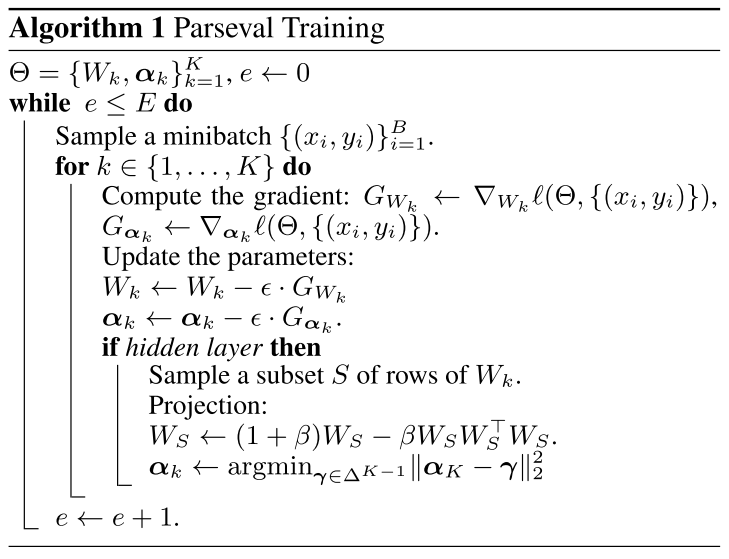
In practice, they use the parseval tightness of weights to regularize them, i.e.
And they actually use two approximations, first by updating only one step for , i.e.
second by sampling a subset of rows and perform the update above, thus reducing the overall complexity to .
To instantiate the convexity constraints in aggregation layers, they project onto postive simplex after a gradient update by
Its solution is of the form .
Denote as the sorted coefficients and , the optimal thresholding is given by
The complexity of the projection is thus .
In short, 1) sort the coefficients of , 2) find a such that is larger than the sum of the largest coefficients, 3) minus the sum of largest coefficients with and divide it by as the , 4) filter the with the calculated threshold .
Experiments
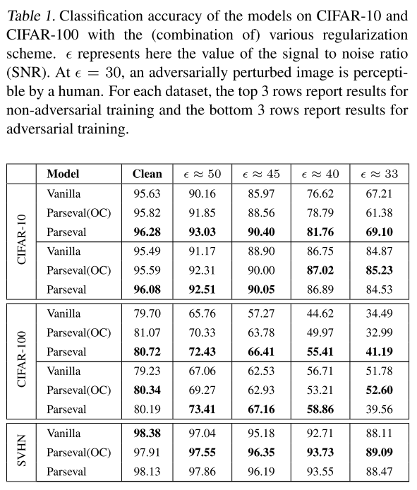
They test Parseval networks on MNIST, CIFAR-10, CIFAR-100 and SVHN.
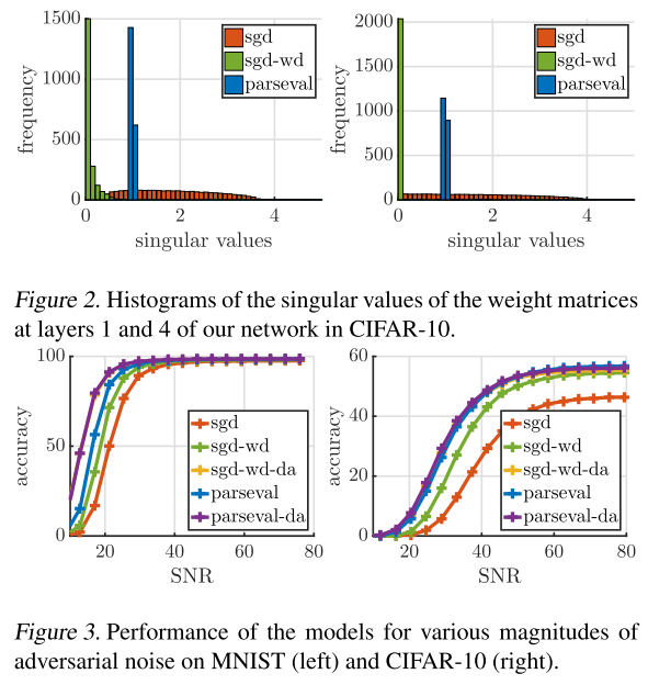
To do so, we analyze the spectrum of the weight matrices of the different models by plotting the histograms of their singular values, and compare these histograms for Parseval networks to networks trained using standard SGD with and without weight decay (SGD-wd and SGD).
They use FGSM to test the robustness and compute the corresponding Signal to Noise Ratio (SNR).i.e. for a perturbation on image
In the table, we denote Parseval(OC) the Parseval network with orthogonality constraint and without using a convex combination in aggregation layers.
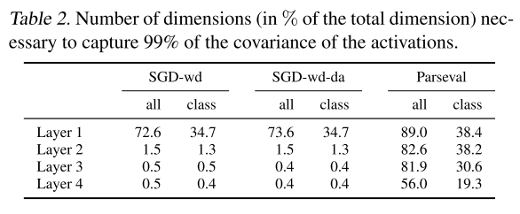
To get Table 2, they compute the activation's empirical covariance matrix for each layer of the fully connected network, i.e.
and obtain its sorted eigenvalues . At last, they select the smallest integer such that .
These results suggest that Parseval contracts the data of each class in a lower dimensional manifold (compared to the intrinsic dimensionality of the whole data) hence making classification easier
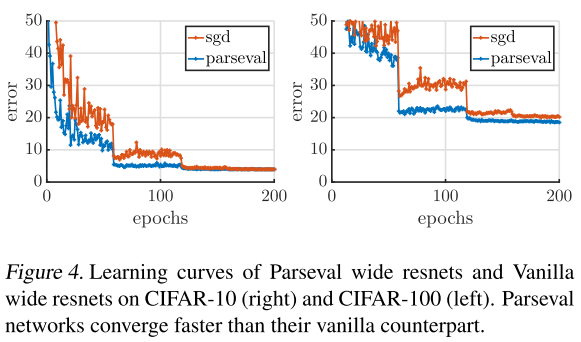
They also observe that Parseval networks coverge signifcantly faster than vanilla conterpart (as shown in Figure 4)
Thanks to the orthogonalization step following each gradient update, the weight matrices are well conditioned at each step during the optimization.
Inspirations
It's a very reasonable idea to constrain the weights to be orthogonal, i.e. make the features learned more diverse, but it seems that the robustness gained by this regularization is limited.
Linear Regularization
Adversarial robustness through local linearization - NIPS 2019
Chongli Qin, James Martens, Sven Gowal, Dilip Krishnan, Krishnamurthy Dvijotham, Alhussein Fawzi, Soham De, Robert Stanforth, and Pushmeet Kohli. Adversarial robustness through local linearization. In NeurIPS, 2019. arXiv:1907.02610
Adversarial training with more attacker steps is stronger but very computationally expensive and that with less attacker steps leads to a phenomenon named as gradient obfuscation, i.e. the gradients around the training example is highly convoluted and complex such that weak attack fails, but the strong attack still succeeds.
However, this can produce models which are robust against weak attacks, but break down under strong attacks – often due to gradient obfuscation
If the loss surface was linear in the vicinity of the training examples, which is to say well-predicted by local gradient information, gradient obfuscation cannot occur.
Adversarial training
A classifier function parameterized by , maps input features to the output logits for classes in set , the probability that the input belongs to class is then calculated using softmax, i.e. . Adversarial robustness for is defined as follows:
A network is robust to adversarial perturbations of magnitude at input if only if
In this paper, they focus on and set , i.e. the -norm attack.
They intend to make improvements based on the adversarial training using PGD, i.e.:
And the inner optimization problem is solved by PGD with each gradient step as:
A naive approach is to reduce the number of gradient steps performed by the optimization procedure. Generally, the attack is weaker when we do fewer steps. If the attack is too weak, the trained networks often display gradient obfuscation as highlighted in Fig 1.
Local linearity measure
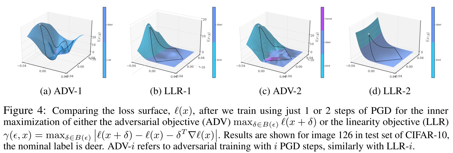
If the loss surface is smooth and approximately linear in input around perturbation , then the loss should be well approximated by its first-order Taylor expansion. Their difference can be an indicator of how linear the loss is:
And for the entire vicinity, we can define a quantity named as local linearity measure:
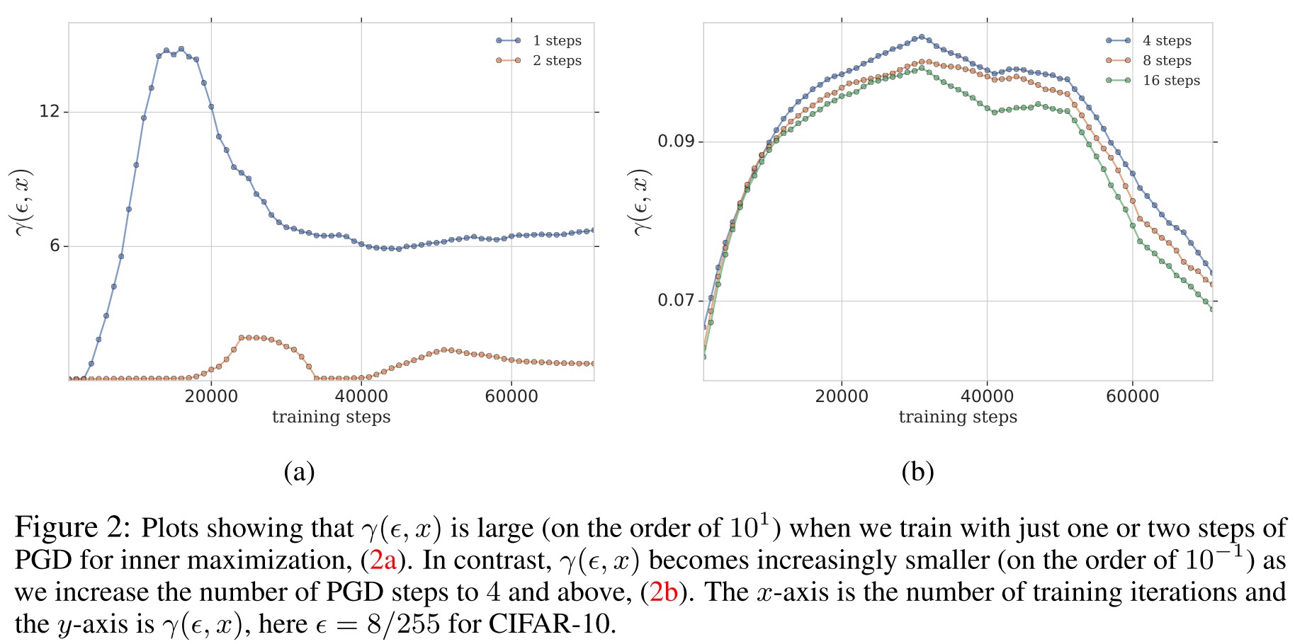
By experiment, they observe that adversarial training with more steps for attacker results a smaller local linearity measure, suggesting that it has a more linear loss surface.
Local linear regularizer (LLR)
Propostition 4.1 Consider a loss function that is once-differentiable, and a local neighborhood defined by . Then for all :
The adversarial loss is upper bounded by the local linearity measure, plus the change in loss as predicted by the gradient.
The adversarial loss tends to , i.e. , as both and for all . (?)
Based on the analysis above, they propose the Local Linearity Regularization (LLR):
In which, , which is a point in where the linear approximation is maximally violated. They penalize both its linear violation and the gradient magnitude term .
The local linearity itself is a sufficient regularizer, but adding a magnitude term makes it better as proved by experiments.
Experiment
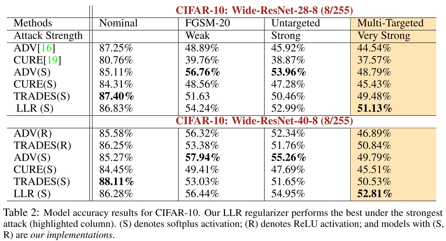
They evaluate LLR on CIFAR-10 and ImageNet:
CIFAR-10
The perturbation radius we examine is = 8/255 and the model architectures we use are Wide-ResNet-28-8, Wide-ResNet-40-8 [29].
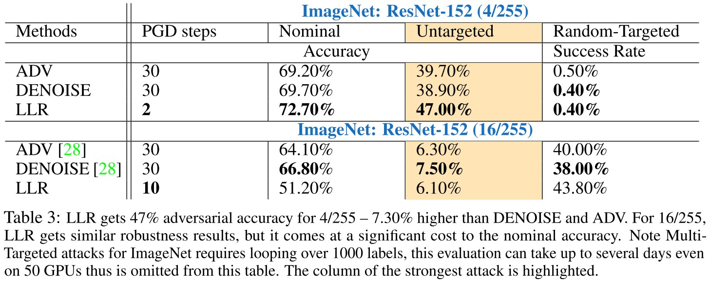
ImageNet
The perturbation radii considered are = 4/255 and = 16/255. The architecture used for this is from [10] which is ResNet-152.
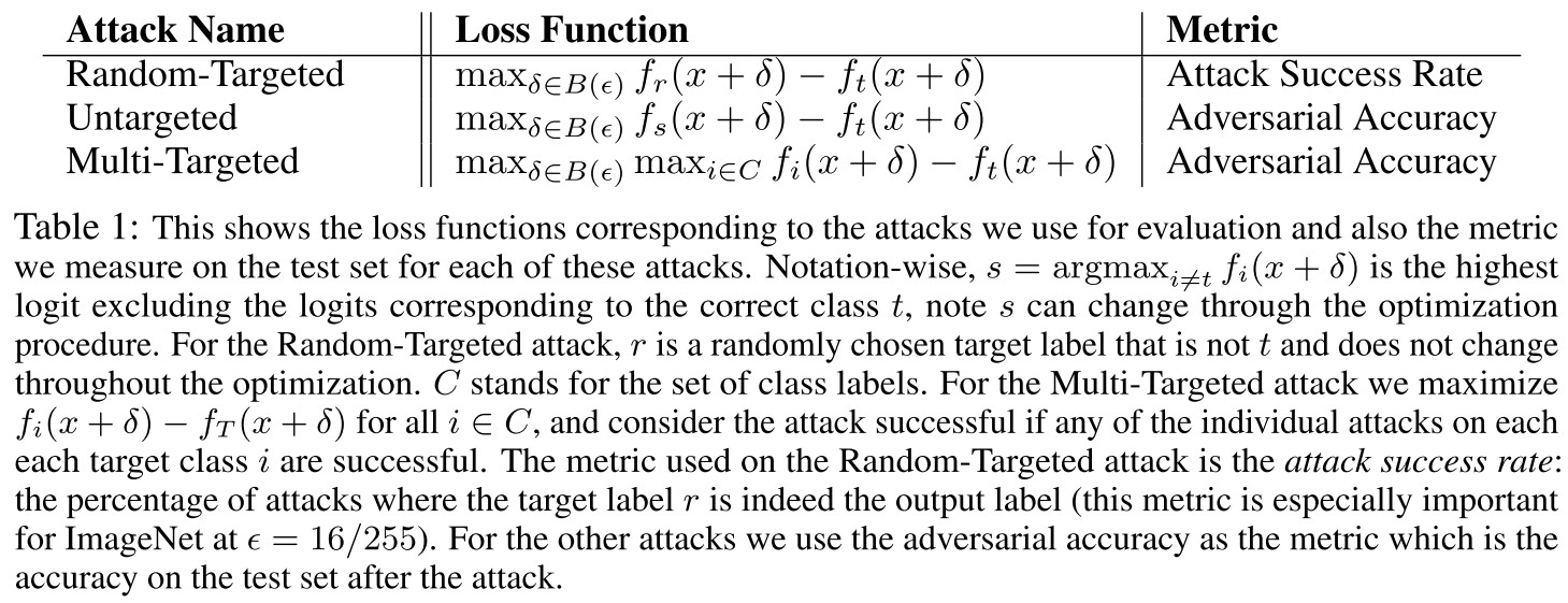
Under three types of attacks:
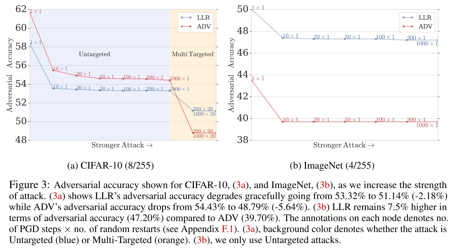
It's also observed that LLR also results a better distribution of robustness over attacks of different strengths:
Logit Regularization
Improved Adversarial Robustness via Logit Regularization Methods - 2019
ICLR 2019 withdrawal
Cecilia Summers, Michael J. Dinneen. Improved Adversarial Robustness via Logit Regularization Methods. arXiv preprint 2019. arXiv:1906.03749
We also demonstrate that much of the effectiveness of one recent adversarial defense mechanism can in fact be attributed to logit regularization, and show how to improve its defense against both white-box and black-box attacks, in the process creating a stronger black-box attack against PGD-based models.
They empirically evaluate a series of logit regularization techniques for their potential to be used as a defense against adversarial attack.
This paper is withdrew by authors, therefore let's read it critically.
In this work, we show that adversarial logit pairing derives a large fraction of its benefits from regularizing the model’s logits toward zero, which we demonstrate through simple and easy to understand theoretical arguments in addition to empirical demonstration.
Adversarial Logit Pairing and Logit Regularization
Adversarial logit pairing refers to pairing the logits activated by adversarial examples and clean examples, i.e. regularizing with
where is the logit of the model for class on clean example , and is the respectively logit of the corresponding adversarial example.
When , this term encourages the original logits to be smaller and adversarial logits to be larger, otherwise reversely, which is essentially regularizing the logits.
If incorporating the shared scale factor , i.e.
implying that
indicating as a global minimizer for the loss. Therefore, adversarial logit pairing also has an effect of logit squeezing.
And it is also demonstrated with experimental results:
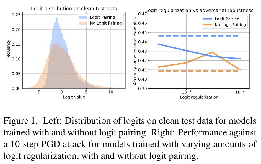
As shown in Figure 1 left, adversarial logit pairing does reduce the magnitude of logits, i.e. showing an effect of logit squeezing and in Figure 1 right, using logit regularization is able to recover slightly more than half of the total improvement from logit pairing.
It's convincing that adversarial logit pairing also squeezes logits, but it's unfortunately that adversarial logit pairing has been demonstrated to be breached.
Label Smoothing
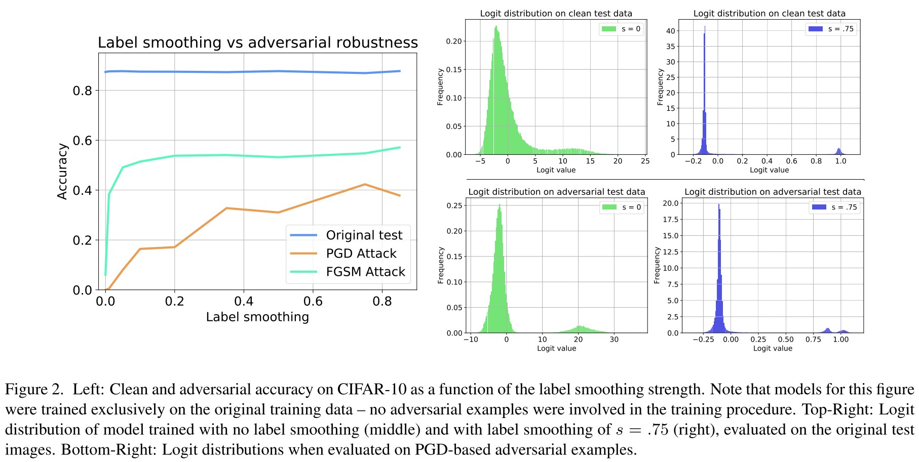
Label Smoothing refers to replacing hard labels with soft labels:
where the number of categories is denoted by and is the smoothing strength.
Interestingly, Kurakin et al. [15] found that incorporating a small amount of label smoothing present in a model trained on ImageNet actually decreased adversarial robustness roughly by 1%.
As shown in Figure 2 left, they discover that aggressive label smoothing can improve adversarial robustness; as shown in Figure 2 right, label smoothing also squeezes the logits, i.e. reducing the dynamic range of logits.
This is also observed in other works.
Other logit regularizations include enforcing linearity both between examples and labels (e.g. mixup).
Decoupling Adversarial Logit Pairing
The regularization term of adversarial logit pairing is
where the first and third terms are explicit logit regularization, and the logit pairing effects is only determined by the middle inner product.
Therefore, the term can be expressed in a more general form:
where the similarity between logits is controlled by a metric .
There are several natural choices for , such as the Jensen-Shannon divergence, a cosine similarity, or any similarity metric that does not have a significant regularization effect.
Their proposal still requires adversarial examples as adversarial training, which is not more computationally efficient.
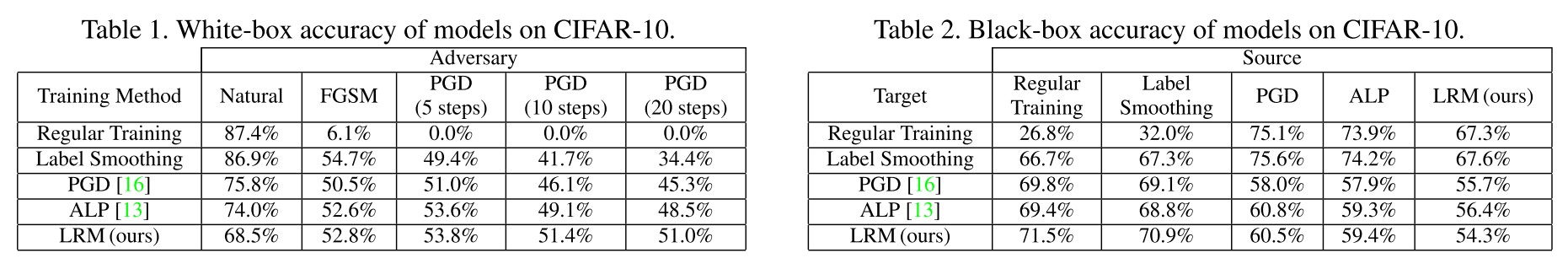
Experiments
Inspirations
It's nice to see that they decoupled adversarial logit pairing and point out the logit squeezing effect of adversarial logit pairing.
Unfortunately, Madry lab has dismissed adversarial logit pairing in 2018 and adversarial logit pairing also shows no promising advantages compared with adversarial training.
In fact, adversarial logit pairing can be seen as a version of adversarial training, the failure of it is quite weird.
Jacobian Regularization
JARN (Jacobian Regularization) - ICLR 2020
Code: https://github.com/alvinchangw/JARN_ICLR2020
Alvin Chan, Yi Tay, Yew Soon Ong, Jie Fu. Jacobian Adversarially Regularized Networks for Robustness. ICLR 2020. arXiv:1912.10185
We propose Jacobian Adversarially Regularized Networks (JARN) as a method to optimize the saliency of a classifier’s Jacobian by adversarially regularizing the model’s Jacobian to resemble natural training images.
Jacobian Adversarially Regularized Networks
The standard cross-entropy loss is
for a classifier and a label as one-hot vector of classes .
With gradient backpropagation to the input layer, through with respect to , the Jacobian matrix is
In which, .
The Jacobians of robust models are empirically observed to be similar to images, and the next part of JARN entails adversarial regularization of Jacobian matrices to induce resemblance with input images.
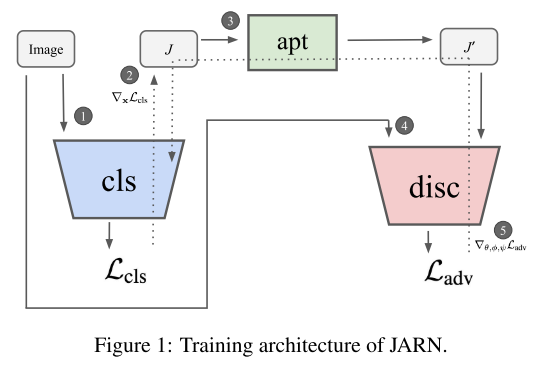
An adaptor network (parameterized with )is introduced to map the Jacobian into the domain of input images, i.e.
The adaptor network and classifier can be framed as a generator
learning to model a distribution that resembles .
A discriminator , parameterized with , that outputs a singla scalar indicating whether the input comes from or is then introduced to form a GAN with . The training of this GAN involves the following adversarial loss
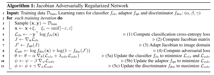
The final loss is a combination of these two losses, and the classifier is learned by
While the optimal parameters for and , i.e. and respectively, are learned by
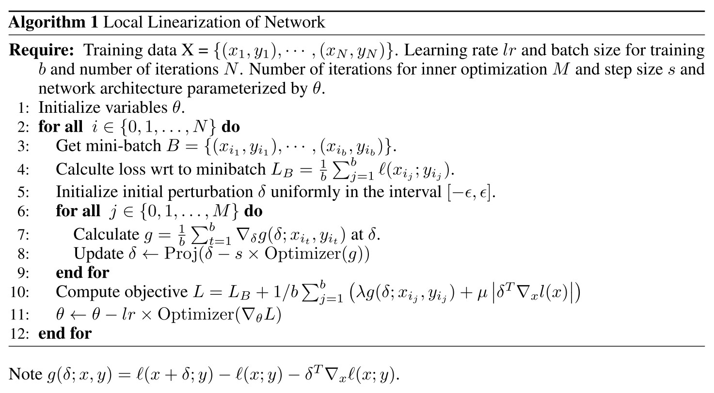
These three networks are optimized simultaneously as shown in Algorithm 1. Similar with GAN, they add some uniformed sampled noise before feeding the to the input.
Theoretical analysis of JARN
Theorem 3.1 The global minimum of is achieved when maps to itself, i.e. .
It's a theorem similar to that in GAN.
In Etmann et al. (2019), it is shown that the linearized robustness of a model is loosely upperbounded by the alignment between the Jacobian and the input image.
Theorem 3.2 (Linearized Robustness Bound) (Etmann et al., 2019) Defining and as top two prediction, we let the Jacobian with respect to the difference in top two logits be . Expressing alignment between the Jacobian with the input as , then
where is a positive constant.
This suggests that a bigger (a Jacobian of more aligned with input ) and a smaller induces a large upper bound of robustness.
Combining with what we have in Theorem 3.1, assuming to be close to in a fixed constant term, the alignment term in Equation (13) is maximum when reaches its global minimum.
Experiments
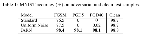
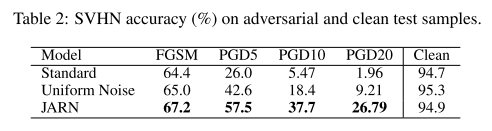
They evaluated their methods on MNIST, SVHN and CIFAR-10, three datasets.
For MNIST:
We train a CNN, sequentially composed of 3 convolutional layers and 1 final softmax layer. All 3 convolutional layers have a stride of 5 while each layer has an increasing number of output channels (64-128-256).
PGD attacks under tolarance of , the uniform noise denotes data augmentation with uniform noise.
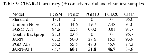
For SVHN and CIFAR-10:
We train the Wide-Resnet model following hyperparameters from (Madry et al., 2017)’s setup for their CIFAR-10 experiments.
PGD attacks under tolarance of .
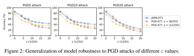
To study how JARN-AT1 robustness generalizes, we conduct PGD attacks of varying ε and strength (5, 10 and 20 iterations).
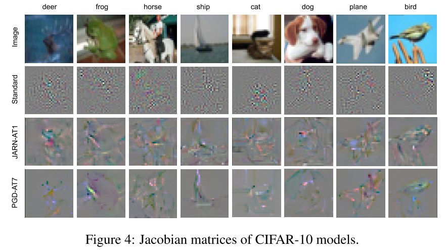
The JARN surely produces Jacobians more similar to the original images.
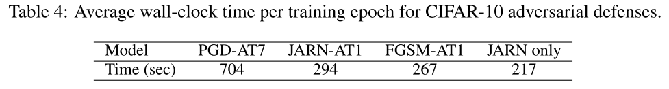
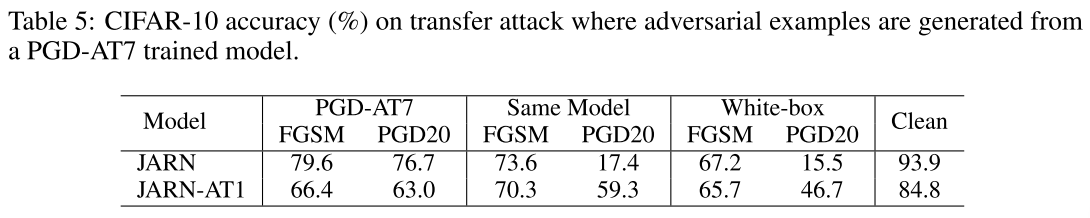
JARN is trained much more fast and it also appears to be more robust to transfer attacks (black-box attacks), which indicates that this is not a method relying on gradient masking.
Inspirations
This paper is a demonstration of the word "research". The empirical works point out the phenomenon, the theoretical works give possible explanation and direction for engineers and the engineering works propose methods to solve the problem.
JARN seems to offer comparable robustness with adversarial training, while using less time. The use of GAN on Jacobians seems a little redundant, perhaps there is some room for improvements.