Explanation for Adversarial Example and Robustness - 2
By LI Haoyang 2020.11.16
Content
Explanation for Adversarial Example and Robustness - 2ContentRobustnessAll-Layer Margin - ICLR 2020 ?Output Margin and GeneralizationNotationSimplified all-layer margin and its guaranteesGeneralization guarantees for neural networksGeneralization guarantees for robust classificationEmpirical application of the all-layer marginInspirationsUnderstanding and Mitigating the Tradeoff Between Robustness and Accuracy - ICML 2020SetupNoiseless linear regressionMinimum norm estimatorsAnalysis in the linear regression settingCase analysisGeneral characterizationsRobust self-trainingRobust self-training in linear regressionEmpirical evaluation of RSTInspirationsAdversarial ExampleAdversarial Examples from Computational Constraints - ICML 2019Excessive Invariance Causes Adversarial Vulnerability - ICLR 2019Two complementary approaches to adversarial examplesUsing bijective networks to analyze excessive invarianceAnalytic attackAttack on adversarial spheresAttack on MNIST and ImageNetIndependence Cross-entropy LossExperimentsInspirationsHold me tight! Influence of discriminative features on deep network boundaries - NIPS 2020Proposed frameworkMargin and discriminative featuresEvidence on synthetic dataEvidence on real dataDiscussionSensitivity to position of training samplesEvidence on synthetic dataConnections to adversarial trainingInspirations
Robustness
All-Layer Margin - ICLR 2020 ?
Paper: https://openreview.net/forum?id=HJe_yR4Fwr
Colin Wei, Tengyu Ma. Improved Sample Complexities for Deep Neural Networks and Robust Classification via an All-Layer Margin. ICLR 2020.
In this work, we propose to instead analyze a new notion of margin, which we call the “all-layer margin.”
Our analysis reveals that the all-layer margin has a clear and direct relationship with generalization for deep models.
Output Margin and Generalization
In linear classifiers, generalization error is controlled by the output margins normalized by the classifier norm.
Suppose there are training data points each with norm , and let be the output margin on the -th example. With high probability, if the classifier perfectly fits the training data, there is
For deeper models, the relationship between output margin and generalization is unfortunately less clear and interpretable.
In this work, we remedy this issue by proposing a new notion of margin, called "all-layer margin", which we use to obtain simple guarantees like (1.1) for deep models.
Let be the all-layer margin for the -th example. A bound can be obtained by simply normalizing it by the sum of the complexities of the weights, formed as following:
They present three applications:
- By relating all-layer margin to output margin and other quantities, we obtain improved generalization bounds for neural nets.
- We extend our tools to give generalization bounds for adversarially robust classification error which are analogous to our bounds in the standard setting.
- We design a training algorithm that encourages a larger all-layer margin and demonstrate that it improves empirical performance over strong baselines.
Notation
They use the following notations:
- , a sequence of elements indexed by .
- , function composition, i.e.
- .
- , partial derivative operator with respect to variable
- , partial derivative of with respect to evaluated at
- , some norm
- , for a function mapping between normed spaces with norms .
- , the Frobenius norms of .
- , the sum of the absolute values of the entries of .
- , the covering number of some set (often a class of functions) in the metric induced by norm with resolution .
- , the covering number of in the metric .
- , where is a function and is a distribution
- , where is a test distribution, denotes inputs and is an integer label.
- is also used to denote the uniform distribution on these training samples.
- , a predicted label on input by a classifier .
- , the 0-1 prediction loss, which outputs 1 when incorrectly classifies and 0 otherwise.
I think the course of functional analysis may be a prerequisite for the understanding of this paper.
Simplified all-layer margin and its guarantees
Popular loss functions for classification, such as logistic and hinge loss, attempt to increase the output margin of a classifier by penalizing predictions that are too close to the decision boundary.
Consider the class multi-class classification setting with a classifier , the output margin on example is defined as
The difference between the correct prediction and the nearest incorrect prediction.
Suppose that the classifier is computed by composing functions , and let denote perturbations intended to be applied at each hidden layer.
The perturbed network output is recursively defined as
The all-layer margin is then defined as the minimum norm of required to make the classifier misclassify the input.
The corresponding perturbation to the input here is also referred as the adversarial robustness of the classifier, i.e. the smallest adversarial perturbation.
For classifier , input and label , it's formulated as
The constraint that misclassifies is equivalent to enforcing . (by definition)
This all-layer margin considers simultaneous perturbations to all layers, which is crucial for achieving its statistical guarantees as they claimed.
Let be the class of compositions of functions from function classes .
An element of , i.e. will be a general classifier.
They assume that the covering number of each layer scales as
for some complexity .
Theorem 2.1 (Simplified version of Theorem A.1) In the above setting, with probability over the draw of the training data, all classifiers which achieve training error 0 satisfy
where is a low-order term.
In other words, generalization is controlled by the sum of the complexities of the layers and the quadratic mean of on the training set.
In favor of generalization, more data (larger ) is better, a larger all-layer margin is better, i.e. more robustness against adversarial perturbation in all layers is better, less complexity is better.
For neural nets, scales with weight matrix norms and can be upper bounded by a polynomial in the Jacobian and hidden layer norms and output margin, allowing us to avoid an exponential dependency on depth when these quantities are well-behaved on the training data.
Lemma 2.1 (Complexity Decomposition Lemma). Let denote the family of all-layer margins of function compositions in . Then
The covering number of an individual layer commonly scales as . In this case, for all , we obtain .
???
Lemma 2.1 shows that the complexity of scales linearly in depth for any choice of layers .
Claim 2.1. For any two compositions and and any , we have
A result by Srebro et al. (2010) shows that generic smooth losses enjoy faster convergence rates if the empirical loss is low.
Lemma 2.2. Suppose that is a -smooth loss function taking values in . Then in the setting of Theorem 2.1, we have with probability for all :
for some universal constant .
???
Generalization guarantees for neural networks
The math is too obscure....
Generalization guarantees for robust classification
Let denote the set of possible perturbation of the adversarial classification loss defined by
Theorem 4.1. Assume that the activation has a -Lipschitz derivative. Fix reference matrices and any integer . With probability over the draw of the training sample , all neural nets which achieve robust training error 0 satisfy
where is defined by for in (3.2), and are defined the same as in Theorem 3.1.
Designing regularizers for robust classification based on the bound in Theorem 4.1 is a promising direction for future work.
Empirical application of the all-layer margin
Inspired by the good statistical properties of the all-layer margin, we design an algorithm which encourages a larger all-layer margin during training.
Let denote the standard cross entropy loss used in training and the parameters of the network, consider the following objective:
This objective can be interpreted as applying the Lagrange multiplier method to a softmax relaxation of the constraint in the objective for all-layer margin.
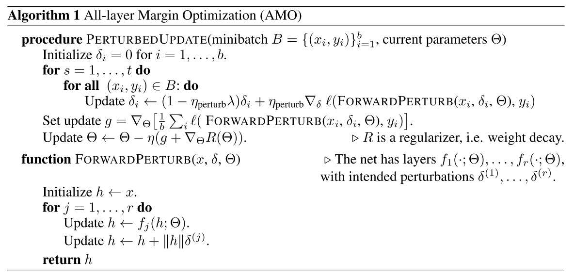
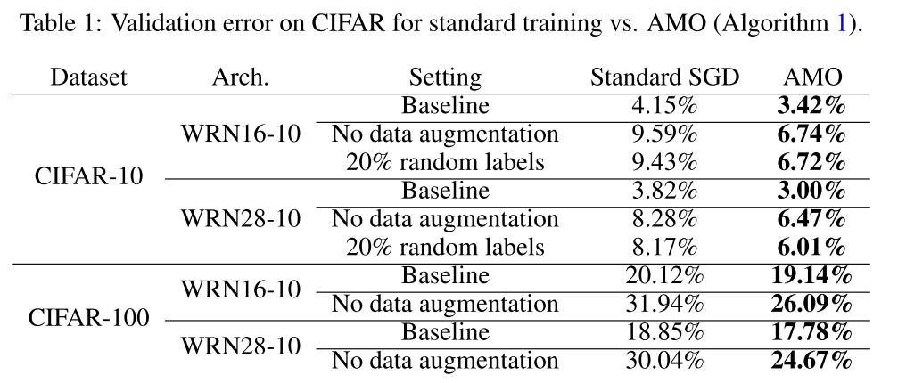
We use Algorithm 1 to train a WideResNet architecture (Zagoruyko and Komodakis, 2016) on CIFAR10 and CIFAR100 in a variety of settings.
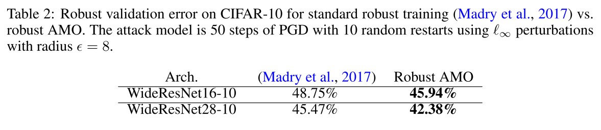
Inspired by our robust generalization bound, we also apply AMO to robust classification by extending the robust training algorithm of (Madry et al., 2017). Madry et al. (2017) adversarially perturb the training input via several steps of projected gradient descent (PGD) and train using the loss computed on this perturbed input.
Inspirations
I do not really get the sense of this paper.....
Understanding and Mitigating the Tradeoff Between Robustness and Accuracy - ICML 2020
Aditi Raghunathan, Sang Michael Xie, Fanny Yang, John Duchi, Percy Liang. Understanding and Mitigating the Tradeoff Between Robustness and Accuracy. ICML 2020. arXiv:2002.10716
Previous works attempt to explain the tradeoff between standard error and robust error in two settings:
- when no accurate classifier is consistent with the perturbed data
- when the hypothesis class is not expressive enough to contain the true classifier
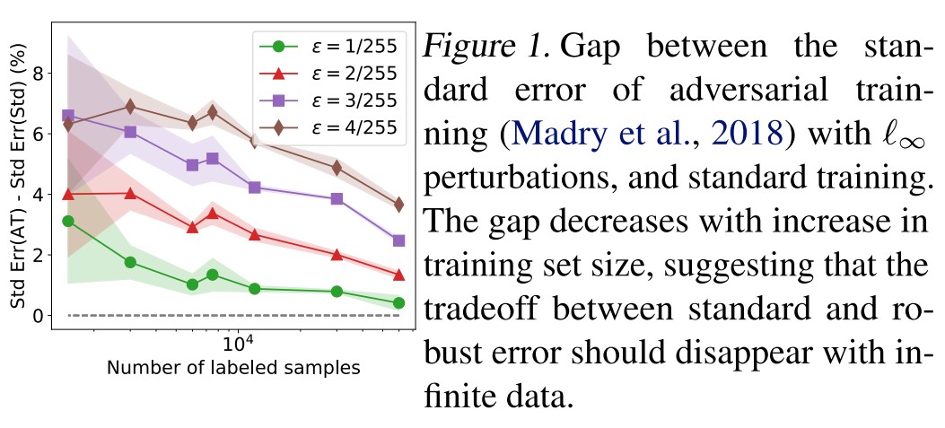
Empirically on CIFAR-10, we find that the gap between the standard error of adversarial training and standard training decreases as we increase the labeled data size, thereby also suggesting the tradeoff could disappear with infinite data (See Figure 1).
In this work, we provide a different explanation for the tradeoff between standard and robust error that takes generalization from finite data into account.
We show that this tradeoff stems from overparameterization. If the restricted hypothesis class (by enforcing invariances) is still overparameterized, the inductive bias of the estimation procedure (e.g., the norm being minimized) plays a key role in determining the generalization of a model.
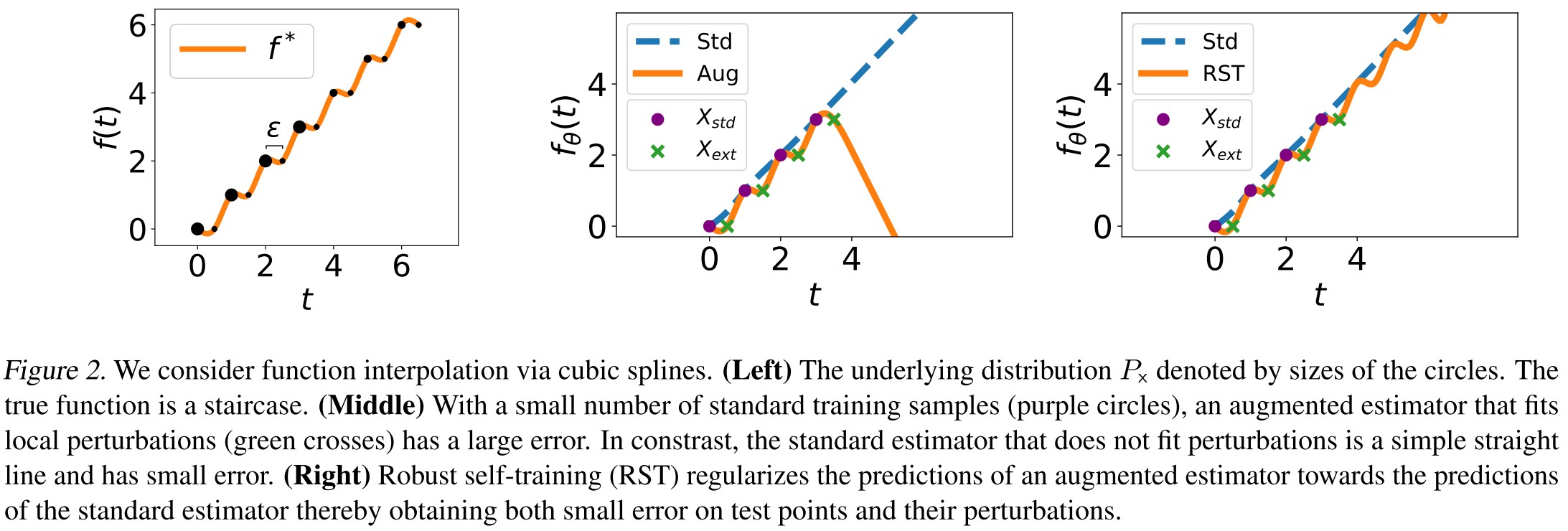
As shown in Figure 2
Training on augmented data with locally consistent perturbations of the training data (crosses) restricts the hypothesis class by encouraging the predictor to fit the local structure of the high density points.
They basically state that adversarial training overfits the augmented data.
Setup
They consider the problem of learning a mapping from input to a target . Theoretically they consider , while empirically they consider general .
The underlying distribution is denoted as , and is the marginal on the inputs, is the conditional distribution of the targets given inputs.
Given training pairs , they use to denote the measurement matrix and to denote the target vector .
The goal is to learn a predictor that has
- low standard error on inputs
- low robust error with respect to a set of perturbations
For a predictor and a loss function , the standard error is
and the robust error is
for consistent perturbations that satisfy
These perturbations should not change the "label" of the target from human perspective.
Noiseless linear regression
For linear regression, i.e. with true parameter , the objective for the standard loss is (squared loss)
where is the population covariance.
Minimum norm estimators
They consider the robust training approaches that augment the standard training data with some extra training data , and call a combination of these two as augmented data.
They compare following mininorm estimators:
The standard estimator interpolating .
The augmented estimator interpolating .
The minimum norm estimators estimate a linear interpolation of the provided data with a minimization of the norm of parameters.
Analysis in the linear regression setting
Case analysis
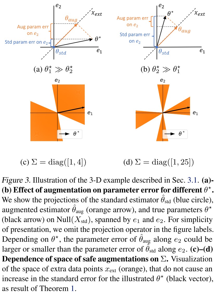
In the 3D space spanned by , and in , suppose there is one data point for standard training .
By definition, there exists , hence , while there is no constraint on the subspace spanned by , i.e. the nullspace , by mininorm objective, the solution is chosen with , as shown in Figure 3, the projection of onto is the blue point at origin.
For this data point, the parameter only fits with the best estimator on the direction of .
Suppose we augment with an extra data point that lies in , as shown in Figure 3, the dotted black line. The augmented estimator still fits the standard data point , i.e. , but with the extra data point , must also satisfy an additional constraint .
The projection of the best estimator onto the extra data point should be the same with that of the augmented estimator.
The crucial observation is that additional constraints along one direction ( in this case) could actually increase parameter error along other directions.
The contribution of different components of the parameter error to the standard error is scaled by the population covariance .
Hence there exists a safe zone that when the augmenting data point falls into this zone, the standard error is not affected.
General characterizations
Define the parameter errors as
The corresponding standard errors are respectively
Define two projection operators respectively
- , the projection matrix onto
- , the projection matrix onto
Since and are minimum norm interpolants, there exist
They should not have any extra value on the nullspace of the given data.
In noiseless linear regression, and have no error in the span of and respectively, i.e.
The parameter error is controlled by the unseen data (the data in the nullspace of given data).
Theorem 1 The difference in the standard errors of the standard estimator and augmented estimator can be written as follows:
where and .
The first term is always positive (as covariance matrix is semidefnite positive), corresponding to the benefit with extra data, while the second term can be negative and intuitively measures the cost of a positive increase in the parameter error along other directions.
The introduced extra data reduces the parameter error in its direction, but may bring other errors in other directions.
Corollary 1 The following conditions are sufficient for , i.e. the standard error does not increase when fitting augmented data.
- The population covariance is identity.
- The augmented data spans the entire space, i.e. .
- The extra data is a single point such that is an eigenvector of .
We would like to draw special attention to the first condition. When , notice that the norm that governs the standard error (Equation 6) matches the norm that is minimized by the interpolants (Equation 5).
As the eigenvalues of become less skewed, the space of safe points expands, eventually covering the entire space when (see Corollary 1).
Propostion 1 For a given ,
for some scalar that depends on .
In other words, for a large increase in standard error upon augmentation, the true parameter needs to be sufficiently more complex (in the norm) than the standard estimator .
Robust self-training
The so-called RST (robust self-training) refers to the adversarial training that incorporates additional unlabeled data via pseudo-labels from a standard estimator.
The general two-step robust self-training procedure is as follows:
- Perform standard training on labeled data to obtain .
- Perform robust training on both the labeled data and unlabeled inputs with pseudo-labels generated from the standard estimator .
The second stage (adversarial training) typically involves a combination of the standard loss and a robust loss , i.e.
On the labeled dataset , the standard and robust loss are
Respectively, on the unlabeled samples , the losses are
Put them together, there comes
for fixed scalars .
Robust self-training in linear regression
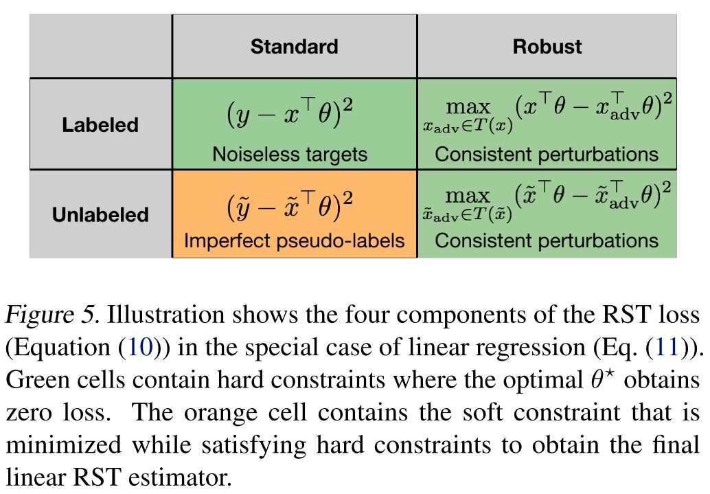
Using the squared loss as the loss function , for consistent perturbations , they analyze the following RST estimator for linear regression
The rest of this section is obscure without any illustration for the .
Empirical evaluation of RST
In this work, we focus on both the standard and robust error and expand upon results from previous work.
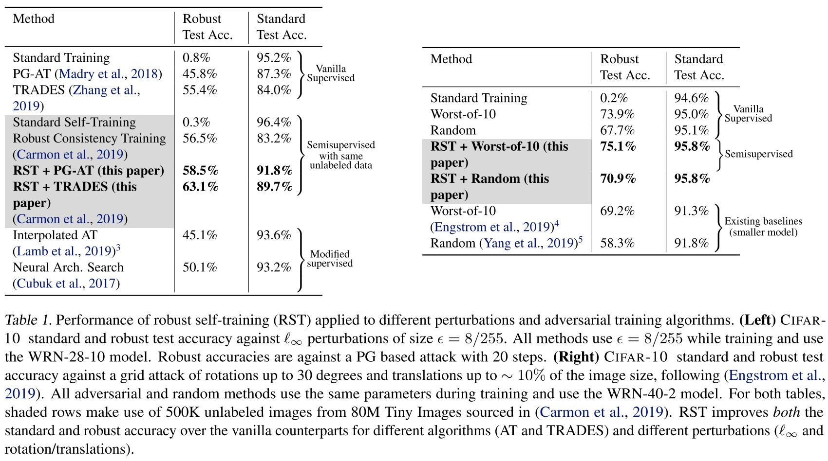
Both RST+AT and RST+TRADES have lower robust and standard error than their supervised counterparts AT and TRADES across all perturbation types.
What is this so-called RST? It's unexpected that there isn't even one table illustrating this algorithm.
By the definition above, it seems that RST here denotes adversarial training with unlabeled data, but it was proposed in Unlabeled data improves adversarial robustness by Carmon et al. in 2019.
What's the difference exactly?
Inspirations
It was great to see someone trying to analyze the tradeoff from different perspectives and the introduction made in this paper showing that it's possible to use RST (robust self-training) without losing much accuracy is also promising.
But the paper itself is too statistical, too many mathematical equations while failed to propose the algorithm or the method clearly....
It's also doubtful whether an analysis on the very simple linear regression can be generalized to the deep models.
Adversarial Example
Adversarial Examples from Computational Constraints - ICML 2019
Sébastien Bubeck, Eric Price, Ilya Razenshteyn. Adversarial examples from computational constraints. ICML 2019. arXiv:1805.10204
Why are classifiers in high dimension vulnerable to “adversarial” perturbations? We show that it is likely not due to information theoretic limitations, but rather it could be due to computational constraints.
Then we give a particular classification task where learning a robust classifier is computationally intractable.
It suggests that adversarial examples may be an unavoidable byproduct of computational limitations of learning algorithms.
Excessive Invariance Causes Adversarial Vulnerability - ICLR 2019
Jörn-Henrik Jacobsen, Jens Behrmann, Richard Zemel, Matthias Bethge. Excessive Invariance Causes Adversarial Vulnerability. ICLR 2019. arXiv:1811.00401
We show deep networks are not only too sensitive to task-irrelevant changes of their input, as is well-known from -adversarial examples, but are also too invariant to a wide range of task-relevant changes, thus making vast regions in input space vulnerable to adversarial attacks.
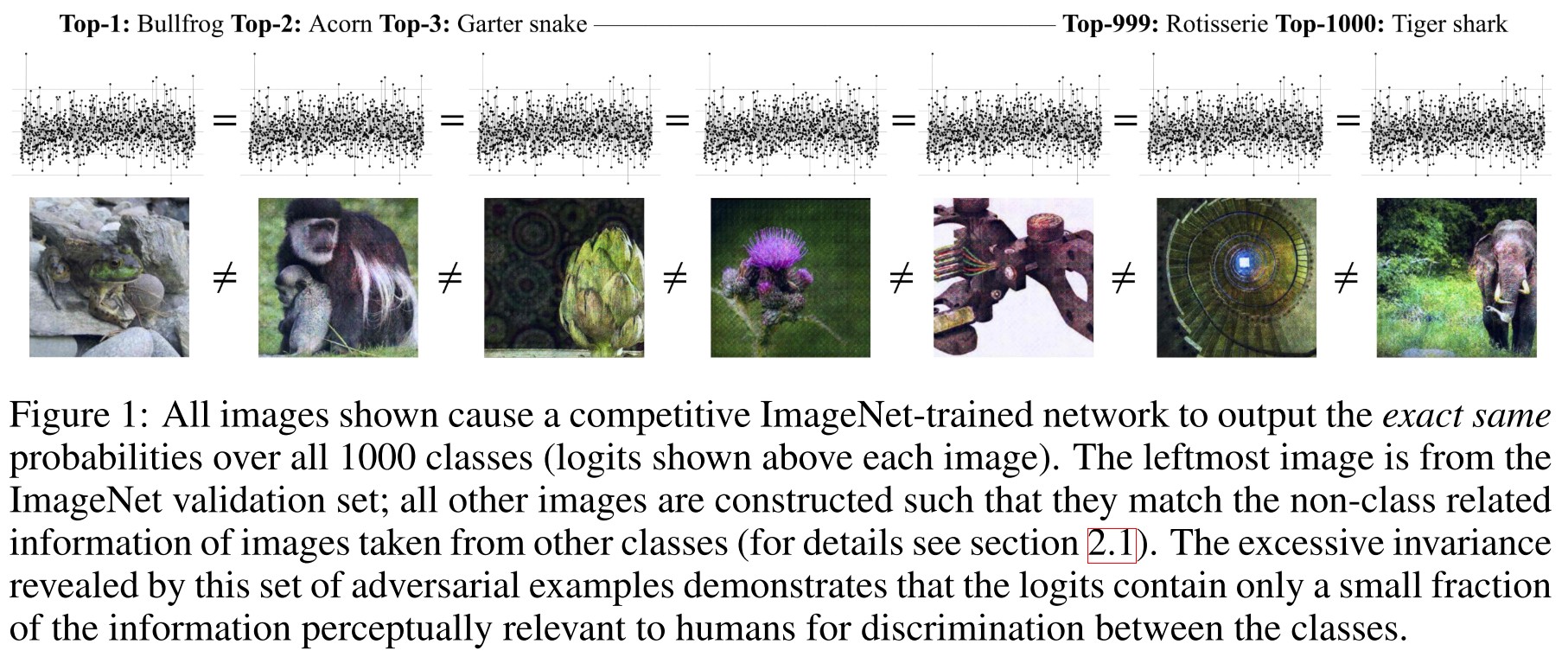
To this end, we introduce the concept of invariance-based adversarial examples and show that class-specific content of almost any input can be changed arbitrarily without changing activations of the network, as illustrated in figure 1 for ImageNet.
The same activation corresponds to many different inputs, therefore, the activations are not even discriminative......
The invariance perspective suggests that adversarial vulnerability is a consequence of narrow learning, yielding classifiers that rely only on few highly predictive features in their decisions.
They point out a complement form of commonly defined adversarial example, i.e. it can also be crafted by keeping the activation unchanged while the content changed drastically.
Two complementary approaches to adversarial examples
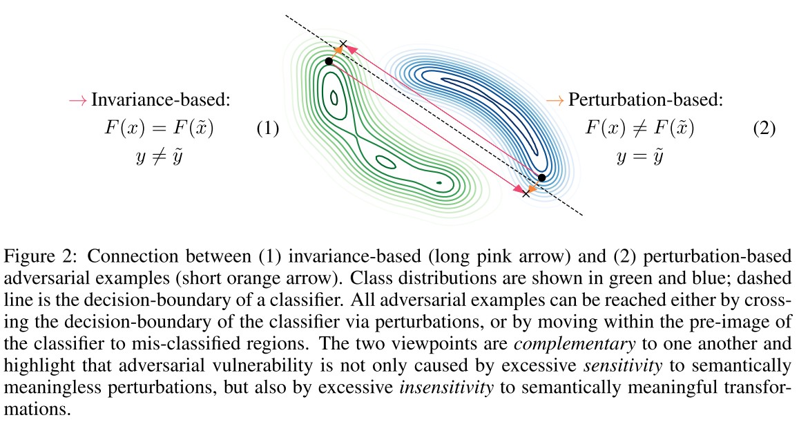
Definition 1 (Pre-images / Invariance). Let be a neural network, with layers and let denote the network up to layer . Further, let be a classifier with . Then for input , we define the following pre-images
- (i) -th Layer pre-image:
- (ii) Logit pre-image:
- (iii) Argmax pre-image:
where by the compositional nature .
Moreover, the (sub-)network is invariant to perturbation which satisfy .
Invariance corresponds to the perturbation that may change the semantic meaning, yet not change the prediction of neural network. The fooling image should stem from the invariance of neural network.
The oracle is a human decision-maker or the unknown input-output function considered in learning theory.
Definition 2 (Perturbation-based Adversarial Examples). A Perturbation-based adversarial example of fulfills:
- Perturbation of decision: and , where is the classifier and is the oracle.
- Created by adversary: is created by an algorithm with .
Further, -bounded adversarial example of fulfill , a norm on and .
This is the generally used definition of an adversarial example.
Definition 3 (Invariance-based Adversarial Examples). Let denote the -th layer, logits or the classifier (Definition 1) and let be in the pre-image of and , an oracle (Definition 2). Then, an invariance-based adversarial example fulfills , while and .
Intuitively, adversarial perturbations cause the output of the classifier to change while the oracle would still consider the new input as being from the original class.
The perturbation-based adversarial examples indicate that the classifier is too sensitive to task-irrelevant changes, while the invariance-based adversarial examples indicate that the classifier is too insensitive to task-relevant changes.
In an unconstrained attack space, these two adversarial examples yield the same input via
with different reference points and , as shown in Figure 2.
Definition 4 (Semantic/Nuisance perturbation of an input). Let be an oracle (Definition 2) and . Then, a perturbation of an input is called semantic, if and nuisance if .
For example, such a nuisance perturbation could be a translation or occlusion in image classification.
The nuisance adversarial example is the generally defined adversarial example, while semantic adversarial example changes the meaning of example, can be viewed as a generative result.
Using bijective networks to analyze excessive invariance
We need a generic approach that gives us access to the discarded nuisance variability.
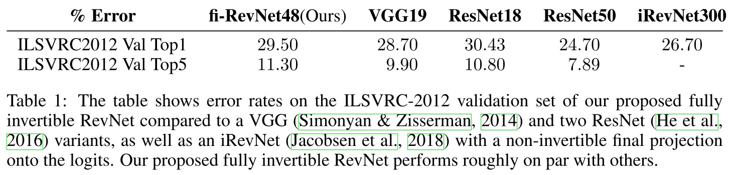
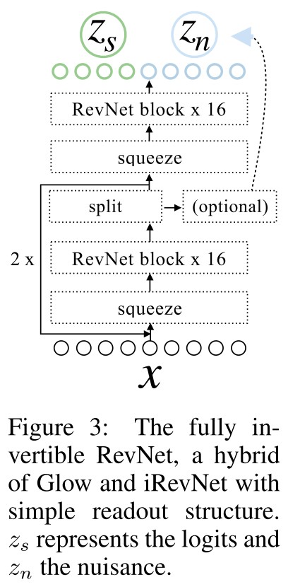
They remove the final linear mapping onto the class probes in invertible RevNet-classifiers and call these networks fully invertible RevNets to gain access to their decision space.
The fully invertible RevNet classifier can be written as
where represents the bijective neural network.
They denote as the logits (semantic variables) and as the nuisance variables ( is not used for classification).
In practice they choose the first indices of the final tensor or apply a more sophisticated DCT scheme.
Due to its simple readout structure, the resulting invertible network allows to qualitatively and quantitatively investigate the task-specific content in nuisance and logit variables.
Analytic attack
The heuristic metameric sampling is obtained by computing , where and are taken from two different inputs.
The samples would be from the true data distribution if the subspaces would be factorized as .
Metameric sampling gives us an analytic tool to inspect dependencies between semantic and nuisance variables without the need for expensive and approximate optimization procedures.
Attack on adversarial spheres
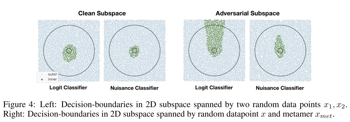
First, we evaluate our analytic attack on the synthetic spheres dataset, where the task is to classify samples as belonging to one out of two spheres with different radii.
We densely sample points in a 2D subspace, following Gilmer et al. (2018b), to visualize two cases:
- 1) the decision-boundary on a 2D plane spanned by two randomly chosen data points,
- 2) the decision-boundary spanned by metameric sample and reference point .
Most notably, the visualized failure is not due to a lack of data seen during training, but rather due to excessive invariance of the original classifier on .
Thus, the nuisance classifier on does not exhibit the same adversarial vulnerability in its subspace.
The nuisance variables are not used for classification, seems naturally immune to adversarial attacks?
Attack on MNIST and ImageNet
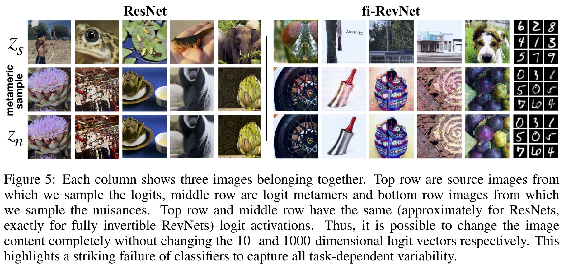
The result is striking, as the nuisance variables are dominating the visual appearance of the logit metamers, making it possible to attach any semantic content to any logit activation pattern.
The attack shows the same failures for non-bijective models. This result highlights the general relevance of our finding and poses the question of the origin of this excessive invariance, which we will analyze in the following section.
Independence Cross-entropy Loss
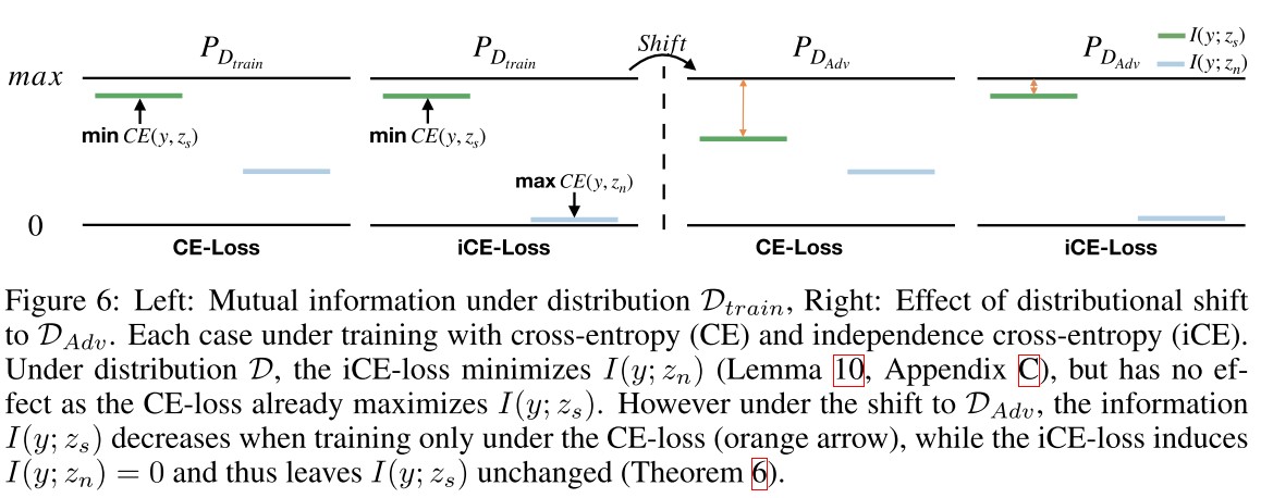
Let with labels . Then the goal of a classifier can be stated as maximizing the mutual information between semantic features (logits) extracted by network and labels , denoted by .
They introduce the concept of an adversarial distribution shift to formalize these modifications brought by these perturbations.
Their first assumption is
i.e. the nuisance variables do not become more informative about .
Thus, the distribution shift may reduce the predictiveness of features encoded in , but does not introduce or increase the predictive value of variations captured in .
Their second assumption is
It corresponds to positive or zero interaction information.
Knowing does not provide more information about .
Bijective networks capture all variations by design, i.e. preserves information
Consider the reformulation
by the chain rule of mutual information.
It offers two ways forward:
- Direct increase of
- Indirect increase of via decreasing
In a general classification task, only is actively increased, which is sufficient in most cases, but may fail under .
Definition 5 (Independence cross-entropy loss). Let a bijective network with parameters and . Furthermore, let be the nuisance classifier with . Then, the independence cross-entropy loss is defined as
The minimization of the nuisance classification loss aims to tighten a lower bound on .
The second term is designed to decrease the mutual information between the target label and nuisance predictions.
Theorem 6 (Information maximal after distribution shift). Let denote the adversarial distribution and the training distribution. Assume by minimizing and the distribution shift satisfies and . Then
Thus, incorporating the nuisance classifier allows for the discussed indirect increase of .
To aid stability, they add a maximum likelihood term to their independence cross-entropy objective, the final term becomes
where denotes the determinant of the Jacobian of and with learned parameters .
Just as in GANs the quality of the result relies on a tight bound provided by the nuisance classifier and convergence of the MLE term.
Experiments
In this section, we show that our proposed independence cross-entropy loss is effective in reducing invariance-based vulnerability in practice by comparing it to vanilla cross-entropy training in four aspects:
- (1) error on train and test set,
- (2) effect under distribution shift, perturbing nuisances via metameric sampling,
- (3) evaluate accuracy of a classifier on the nuisance variables to quantify the class-specific information in them and
- (4) on our newly introduced shiftMNIST, an augmented version of MNIST to benchmark adversarial distribution shifts according to Theorem 6.
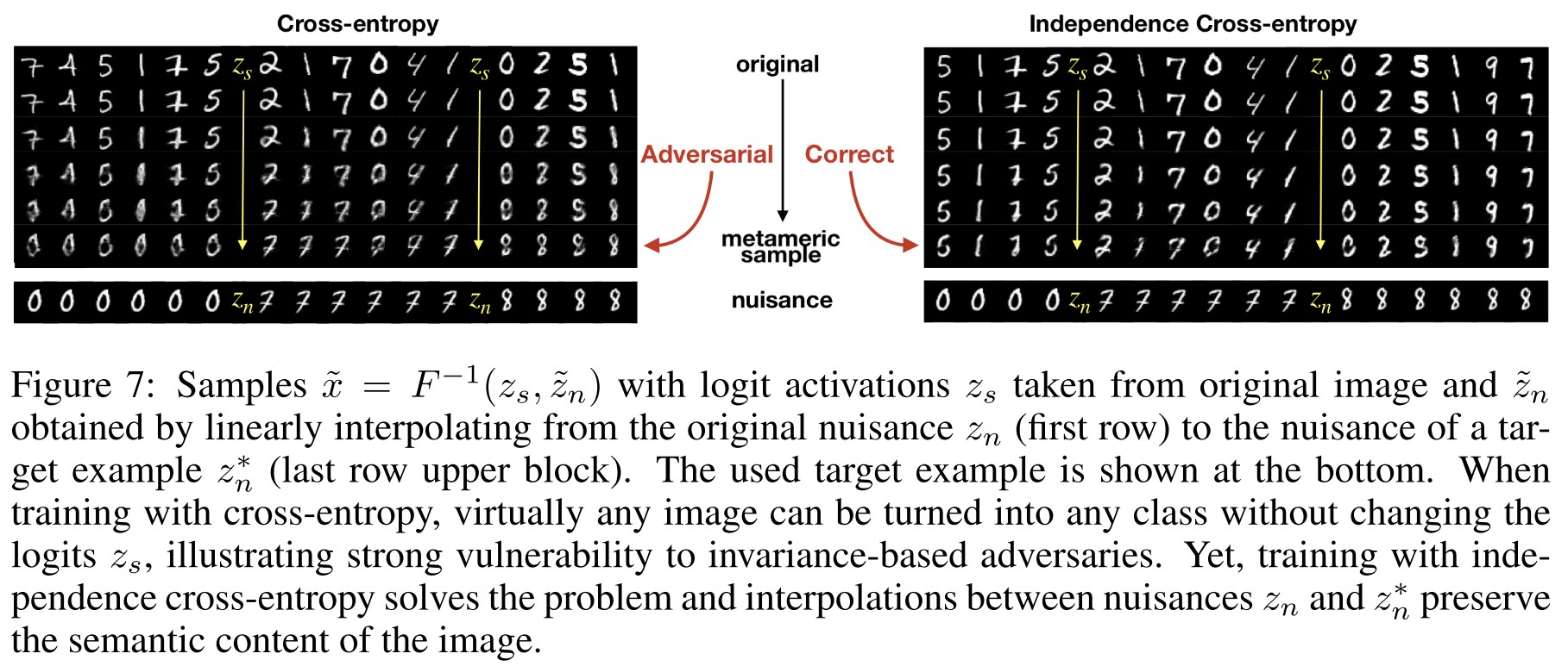
The CE-trained network allows us to transform any image into any class without changing the logits. However, when training with our proposed iCE, the picture changes fundamentally and interpolations in the pre-image only change the style of a digit, but not its semantic content.
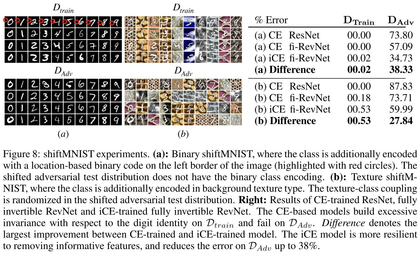
To further test the efficacy of our proposed independence cross-entropy, we introduce a simple, but challenging new dataset termed shiftMNIST to test classifiers under adversarial distribution shifts.
The dataset is based on vanilla MNIST, augmented by introducing additional, highly predictive features at train time that are randomized or removed at test time.
It turns out that this task is indeed very hard for standard classifiers and their tendency to become excessively invariant to semantically meaningful features, as predicted by our theoretical analysis.
When trained with cross-entropy, ResNets and fi-RevNets make zero errors on the train set, while having error rates of up to 87% on the shifted test set.
When applying our independence cross-entropy, the picture changes again. The errors made by the network improve by up to almost 38% on binary shiftMNIST and around 28% on textured shiftMNIST.
Inspirations
This paper presents an important complementary type of adversarial examples, pointing out that invariance to semantically meaningful features also leads to weak adversarial robustness to the model.
The basic idea is the same as that in fooling image, but they rephrase it into an easy term and make more theoretically sound analysis. They further propose a new loss and experiments show its effectiveness, although I see it as a little fuzzy.
It's a promising direction to combine bijective network and adversarial robustness.
Hold me tight! Influence of discriminative features on deep network boundaries - NIPS 2020
Code: https://github.com/LTS4/hold-me-tight
Guillermo Ortiz-Jimenez, Apostolos Modas, Seyed-Mohsen Moosavi-Dezfooli, Pascal Frossard. Hold me tight! Influence of discriminative features on deep network boundaries. NIPS 2020. arXiv:2002.06349
In this work, we borrow tools from the field of adversarial robustness, and propose a new perspective that relates dataset features to the distance of samples to the decision boundary.
Finally, we show that the construction of the decision boundary is extremely sensitive to small perturbations of the training samples, and that changes in certain directions can lead to sudden invariances in the orthogonal ones.
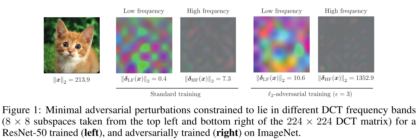
Clearly, reaching the boundary using high frequency perturbations requires much more energy than using low frequency ones [7].
But surprisingly, when the network is adversarially trained [5], the largest increase in margin happens in the high frequency subspace.
Adversarial training dramatically increase the robustness of model against high frequency perturbations.
They intend to answer two questions in this paper:
- How is the margin in different directions related to the features in the training data?
- How can very small perturbations significantly change the geometry of deep networks?
Proposed framework
For a neural network
where is the -th component of the logits of the network .
The decision boundary between classes and of a neural network is the set
In this work, they study the role of training set on the boundary .
Definition 1 (Minimal adversarial perturbations). Given a classifier , a sample , and a sub-region of the input , we define the () minimal adversarial perturbation of in as .
In general, denotes .
The minimal norm of adversarial perturbations reachable in the given region.
Definition 2 (Margin) The magnitude is the margin of in .
The main objective is to obtain a local summary of around a set of observation samples by measuring their margin in a sequence of distinct subspaces .
Given a set of samples, the purpose is to obtain their distances to the boundary by constructing adversarial perturbations.
They use DeepFool attack for further research.
Margin and discriminative features
We want to show that neural networks only construct boundaries along discriminative features, and that they are invariant in every other direction.
Evidence on synthetic data
They generate a balanced training set by independently sampling points , such that and , where denotes the concatenation operator, the feature size and .
The labels are uniformly sampled from . is a random orthonormal matrix, multiplied to avoid an y possible bias of the classifier towards the canonical basis.
Note that this is a linearly separable dataset with a single discriminative feature parallel to (i.e., first row of ), and all other dimensions filled with non-discriminative noise.
They synthesize a dataset that only one discriminative feature is included.
To evaluate our hypothesis, we train a heavily overparameterized multilayer perceptron (MLP) with 10 hidden layers of 500 neurons using SGD (test: 100%)
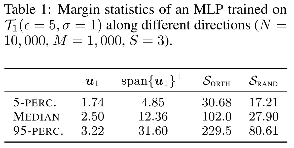
They then calculate the margin statistics on
- the linearly separable direction
- its orthogonal complement
- a fixed random subspace of dimension , i.e.
- a fixed random subspace of the same dimensionality, but orthogonal to , i.e.
As shown in Table 1
From these values we can see that along the direction where the discriminative feature lies, the margin is much smaller than in any other direction.
Evidence on real data
In our study, we train multiple networks on MNIST [25] and CIFAR-10 [26], and for ImageNet [27] we use several of the pretrained networks provided by PyTorch [28].
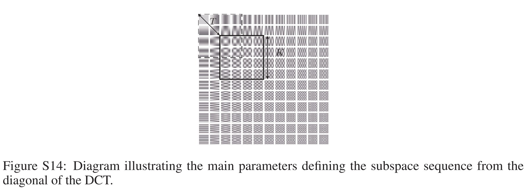
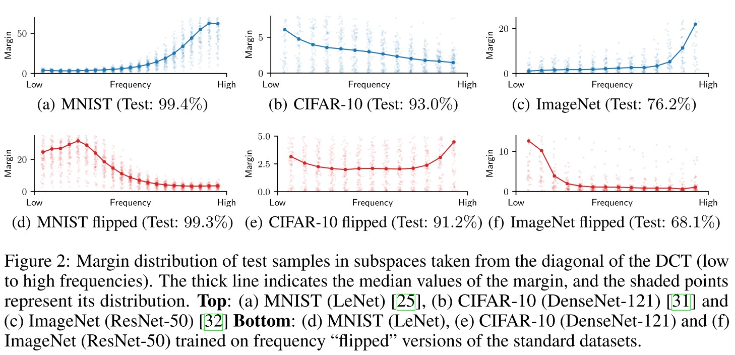
Let denote the width, height and number of channels of the images in those datasets respectively. They use the 2-dimensional discrete cosine transform (2D-DCT) basis of size to generate the observation subspaces .
Let denote the 2D-DCT generating tensor, such that represents one basis element of the image space. The subspaces are generated by sampling blocks from the diagonal of the DCT tensor using a sliding window with step-size .
A more aligned basis with respect to the discriminative features would probably show a sharper transition between low and high margins.
For MNIST and ImageNet, the networks present a strong invariance along high frequency directions and small margin along low frequency ones.
Notice, however, that for CIFAR-10 dataset the margin values are more uniformly distributed; an indication that the network exploits discriminative features across the full spectrum as opposed to the human vision system [33].
This discovery is very interesting. However, it may be caused by the model, rather than the dataset itself.
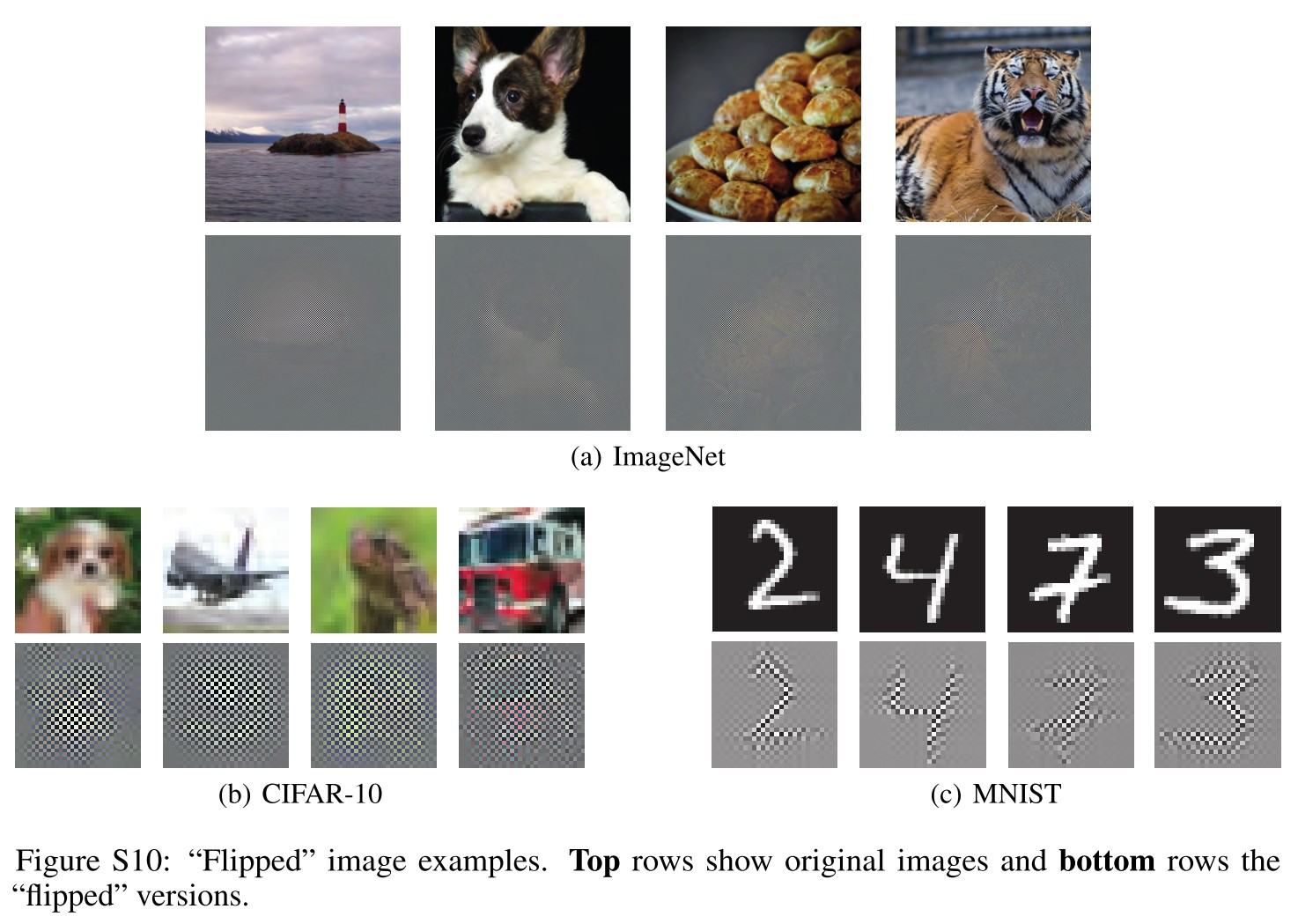
The "flip" operation tweak the distribution of information along the spectrum, particularly, the filpped image of is acquired by
where is the DCT transform and corresponds to one horizonal and one vertical flip of the DCT transformed image.
As shown in Figure 2 bottom,
For both MNIST and ImageNet, the directions of the decision boundaries indeed follow the new data representation – although they are not an exact mirroring of the original representation.
Note again that for CIFAR-10 the effect is not as obvious, due to the quite uniform distribution of the margin.
In order to verify that the small margins in Figure 2 do correspond to directions containing discriminative features, they explicitly modify the features of CIFAR-10 to induce a desired margin.
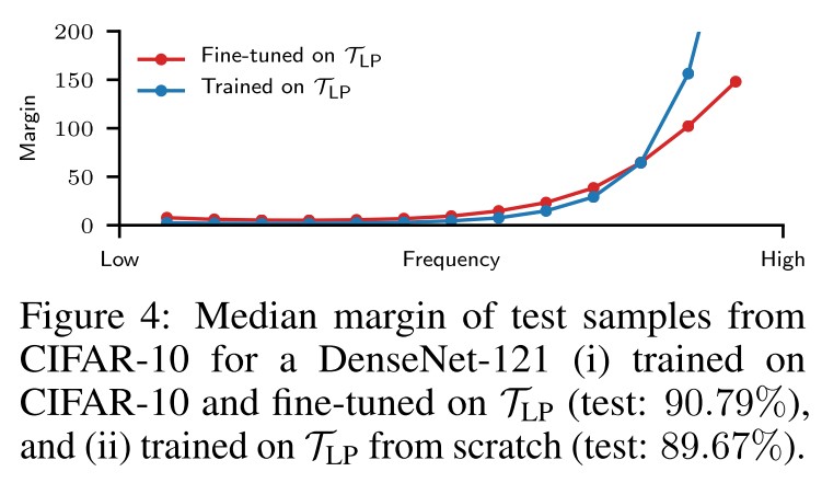
They create a low-pass filtered version of CIFAR-10 () by retaining only the frequency components in a square at the top left of the diagonal of the DCT-transformed images.
As shown in Figure 4,
Indeed, by eliminating the high frequency content, we have forced the network to become invariant along these directions.
Moreover, this effect can also be triggered during training. To show this, we start with the CIFAR-10 trained network studied in Fig. 2(b) and continue training it for a few more epochs with a small learning rate using only .
The elasticity to the modification of features during training gives a new perspective to the theory of catastrophic forgetting [34], as it confirms that the decision boundaries of a neural network can only exist for as long as the classifier is trained with the features that hold them together.
This part can be related to that in Understanding and Mitigating the Tradeoff Between Robustness and Accuracy, where they analyze a simple scenario in 3D space.
Discussion
The main claim in this section is that deep neural networks only create decision boundaries in regions where they identify discriminative features in the training data.
Interesting, but not surprising. You cannot require someone to do well on something completely unseen.
In particular, there are two main confounding factors that might alternatively explain our results: the network architecture or the training algorithm.
However, the experiments in Sec. 3.2 are precisely designed to rule out their influence in this phenomenon.
I don't think they rule them out.....
Sensitivity to position of training samples
In this section, we use it to explain how training with a slightly perturbed version of the training samples can greatly alter the network geometry.
Evidence on synthetic data
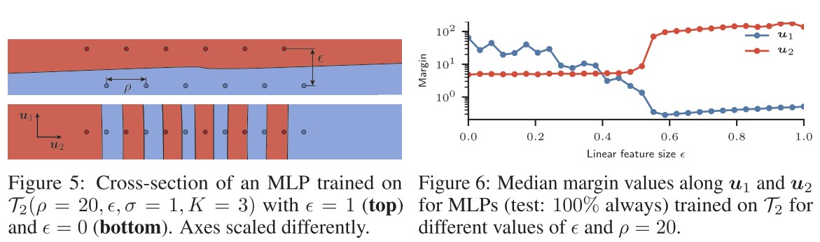
They use a family of training sets consisting in independent -dimensional samples , such that
The feature sizes are controlled by , and for , this training set is always linearly separable.
Fig. 6 shows the median margin values of observation samples for an MLP trained on different versions of with a fixed , but a varying small .
As shown in Figure 6, when the linearly separable feature is small, the model mainly use the non-linear alternative feature , but when the former is larger enough, the model suddenly switch to .
We conjecture that this phenomenon is rooted on the strong inductive bias of the learning algorithm to build connected decision regions whenever geometrically and topologically possible, as empirically validated in [15].
Connections to adversarial training
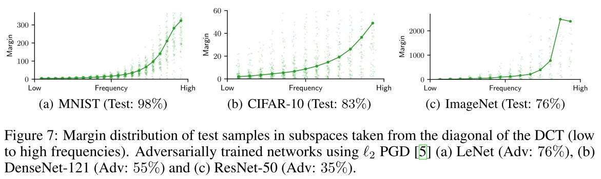
As expected, the margins of the adversarially trained networks are significantly higher than those in Fig. 2.
Surprisingly, though, the largest increase can be noticed in the high frequencies for all datasets.
They conduct some experiments on CIFAR-10 to probe the dynamics of this process.
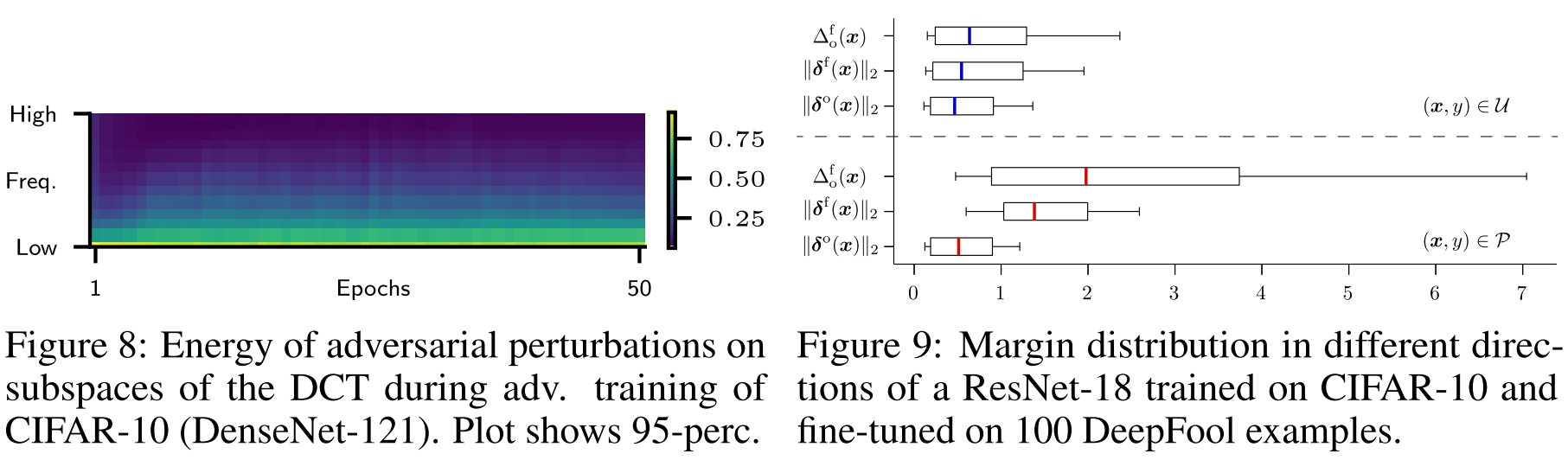
Adversarial perturbations can trigger invariance in orthogonal directions
Fig. 8 shows the spectral decomposition of the adversarial perturbations crafted during adversarial training of CIFAR-10.
However, the greatest effect on margin is seen on the orthogonal high frequency directions (see Fig. 7).
Overall, we see that adversarial training exploits the sensitivity of the network to small changes in the training samples to hide some discriminative features from the model.
A -norm perturbation used for adversarial training restricts the dual norm -norm of the gradients, how similar.
Invariance can be triggered by just a few samples
As shown in Figure 9
Modifying the position of just a minimal number of training samples is enough to locally introduce excessive invariance on a classifier.
This means that modifying the position of only a small fraction of the training samples can induce a large change in the shape of the boundary.
Not very exciting discovery....
Inspirations
This paper utilizes adversarial attack as a tool to research the decision boundary of deep models.
It provides hard evidence that current adversarial training significantly biased to making the model more invariance to high frequency components, i.e. more sensitive to low frequency components, which was also empirically observed and utilized by other works.
One of the interesting phenomenon unaddressed is that they discover that the DenseNet trained on CIFAR-10 appeals to utilize both high frequency and low frequency information uniformly, it may have some connection to the discovery made by NAS for robustness that a densely connected network is relatively more robust.
Besides, their conclusion is not complete architecture agnostic and training algorithm agnostic, which I believe as a future task worth exploring.