Explanation for Robustness and Adversarial Example - 1

By LI Haoyang 2020.10

Robustness

This direction germinates from the robustness analysis of machine learning algorithms, which is a domain with a long history.

Robustness of classifiers: from adversarial to random noise - NIPS 2016

Paper: https://dl.acm.org/doi/abs/10.5555/3157096.3157279

Alhussein Fawzi, Seyed-Mohsen Moosavi-Dezfooli, and Pascal Frossard. 2016. Robustness of classifiers: from adversarial to random noise. In Proceedings of the 30th International Conference on Neural Information Processing Systems (NIPS'16). Curran Associates Inc., Red Hook, NY, USA, 1632–1640. arXiv:1608.08967

In the random regime, we show that the robustness of classifiers behaves as $\sqrt{d}$ times the distance from the datapoint to the classification boundary (where d denotes the dimension of the data) provided the curvature of the decision boundary is sufficiently small.

We show that the robustness precisely behaves as $\sqrt{d/m}$ times the distance to boundary, with $m$ as the dimension of the subspace. This result shows in particular that, even when $m$ is chosen as a small fraction of the dimension $d$, it is still possible to find small perturbations that cause data misclassification.

Definitions and notations

For a $L$-class classifier $f:\Bbb{R}^d\to \Bbb{R}^L$, given a datapoint $x_0\in \Bbb{R}^d$, the estimated label is obtained by $\hat{k}(x_0)=\mathop{\arg\max}_kf_k(x_0)$. Let $\cal{S}$ be an arbitrary subspace of $\Bbb{R}^d$ of dimension $m$.

The adversarial perturbation $r_\cal{S}^*$ is a perturbation of minimal norm in $\cal{S}$ that is required to change the estimated label of $f$ at $x_0$:

It can also be equivalently written as:

When $\cal{S}=\Bbb{R}^d$ and $r^*(x_0)=r_{\Bbb{R}^d}^*(x_0)$ is the generally defined adversarial perturbation.

The robustness of $f$ at $x_0$ along $\cal{S}$ is naturally measured by the norm $||r_{\cal{S}}^*(x_0)||_2$. Different choices of $\cal{S}$ corresponds to study in different regimes:

• Random noise regime

  The robustness quantity in this regime is defined as:

  $$\min_t|t|\ s.t.\ \exist k\ne \hat{k}(x_0),f_k(x_0+tv)\ge f_{\hat{k}(x_0)}(x_0+tv)$$

  In which, $t$ is sampled from one-dimensional subspace $\cal{S}$ with direction $v$ , which is a vector sampled uniformly at random from the unit sphere $\Bbb{S}^{d-1}$ of $d$ dimensions.

• Semi-random noise regime

  In this case, the subspace $\cal{S}$ is chosen randomly, but can be arbitrary dimension $m$. When $m$ is one, it reduces to random noise regime.

In short, the random noise regime perturbs the original input with a noise vector $v$ sampled uniformly from unit sphere with amplitude $t$, the semi-random noise regime expands the amplitude into a vector of arbitrary dimension $m$.

Robustness of clasifiers

Affine classifiers

Assume $f$ is an affine classifier, i.e.:

Theorem 1 Let $\delta>0$ and $\cal{S}$ be a random $m$-dimensional subspace of $\Bbb{R}^d$, and $f$ be a $L$-class affine classifier. Let

The following inequalities hold between the robustness to semi-random noise $||r_{\cal{S}}^*||2$ , and the robustness to adversarial perturbations $||r^*||_2$:

with probability exceeding $1-2(L+1)\delta$.

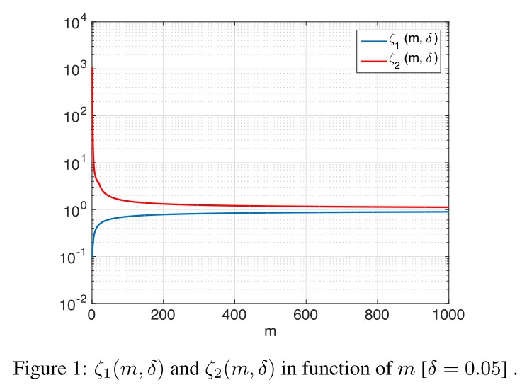
It shows that in the random and semi-random noise regimes, the robustness to noise is precisely related to $||r^*||_2$ by a factor of $\sqrt{d/m}$.

Our results therefore show that, in high dimensional classification settings, affine classifiers can be robust to random noise, even if the datapoint lies very closely to the decision boundary (i.e. $||r^*||_2$ is small).

In the semi-random regime with $m$ sufficiently large (e.g. $m\ge 250$), we have $||r_{\cal{S}}^*||_2\approx\sqrt{d/m}||r^*||_2$ with high probability, as the constants $\zeta_1(m,\delta)\approx\zeta_2(m,\delta)\approx 1$ for sufficiently large $m$.

General classifiers

Curvature of decision boundary

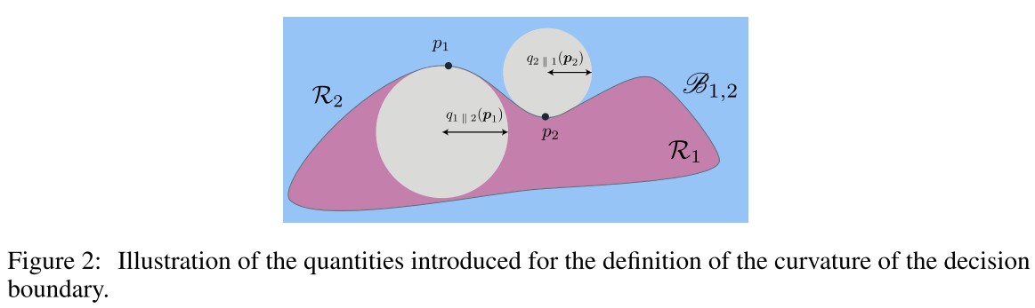
For a general binary classifier, the decision boundary $\scr{B}_{i,j}$ between two classes $i$ and $j$ is:

The two regions separated by this boundary, $\cal{R}_i$ and $\cal{R}_j$, where the estimated label is respectively $i$ and $j$:

For a given $p\in \scr{B}_{i,j}$, we define $q_{i||j}(p)$ to be the radius of the largest open ball included in the region $\cal{R}_i$ that intersects with $\scr{B}_{i,j}$ at $p$, i.e.:

In which, $\Bbb{B}(z,||z-p||_2)$ is the open ball in $\Bbb{R}^d$ of center $z$ and radius $||z-p||_2$.

In human words, it's defined as the radius of the biggest ball intersecting the point $p$ on the boundary, while the ball itself falls completely in one side of the boundary.

This definition is asymmetric, therefore, a symmetric quantity $q_{i,j}(p)$ is defined to be the radius of the worst-case ball inscribed in any of the two regions:

From one point $p$ to the entire boundary, the global curvature is defined as the worst case radius over the entire boundary :

The curvature $\kappa(\scr{B}_{i,j})$ is simply defined as the inverse of the worst-case radius over all points $p$ on the decision boundary.

In the case of affine classifiers, we have $\kappa(\scr{B}_{i,j})=0$, as it's possible to inscribe balls of infinite radius inside each region of the space.

In general, the quantity $\kappa(\scr{B}_{i,j})$ provides an intuitive way of describing the nonlinearity of the decision boundary by fitting balls inside the classification regions.

Robustness to random and semi-random noise

For a binary classification problem, where only classes $\hat{k}$ and $k\in\{1,\dots,L\}\backslash\{\hat{k}\}$ are considered, and $\scr{B}_k:=\scr{B}_{k,\hat{k}}$ be the decision boundary between classes $k$ and $\hat{k}$, the semi-random robustness and adversarial robustness defined above can be re-written as:

Theorem 2 Let $\cal{S}$ be a random $m$-dimensional subspace of $\Bbb{R}^d$. Let $\kappa:=\kappa(\scr{B}_k)$. Assuming that the curvature satisfies

the following inequality holds between the semi-random robustness $||r_{\cal{S}}^k||_2$ and the adversarial robustness $||r^k||_2$:

with probability larger than $1-4\delta$. The constants are $C=0.2$,$C_1=0.625$,$C_2=2.25$.

This result shows that the bounds relating the robustness to random and semi-random noise to the worst-case robustness can be extended to nonlinear classifiers, provided the curvature of the boundary $\kappa(\scr{B}_k)$ is sufficiently small.

The set $A$ is a set of excluded classes $k$ where $||r^k||_2$ is large:

These excluded classes are those with no boundary with class $\hat{k}$.

Assuming a curvature constraint only on the close enough classes, the following result establishes a simplified relation between $||r_{\cal{S}}^*||_2$ and $||r^*||_2$.

Corollary 1 Let $\cal{S}$ be a random $m$-dimensional subspace of $\Bbb{R}^d$. Assume that, for all $k\notin A$, we have

Then, we have

with probability larger than $1-4(L+2)\delta$.

In particular, $||r_{\cal{S}}^*||_2$ is precisely related to the adversarial robustness $||r^*||_2$ by a factor of $\sqrt{d/m}$.

In the random regime ($m=1$), this factor becomes $\sqrt{d}$, and shows that in high dimensional classification problems, classifiers with sufficiently flat boundaries are much more robust to random noise than to adversarial noise.

In other words, if a classifier is highly vulnerable to adversarial perturbations, then it is also vulnerable to noise that is overwhelmingly random and only mildly adversarial (i.e. worst-case noise sought in a random subspace of low dimensionality $m$).

Experiments

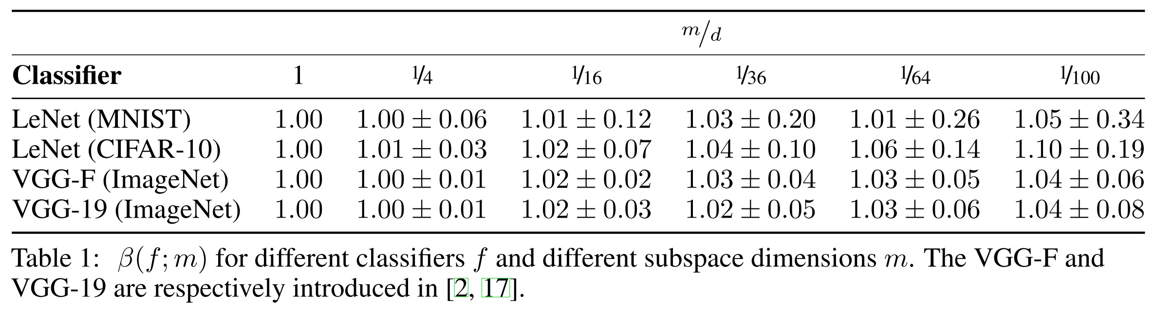
The $\beta(f;m)$ is defined as:

In which, $\scr{D}$ denotes the test set and $\cal{S}$ is chosen randomly for each sample $\boldsymbol{x}$.

This quantity provides indication to the accuracy of the proposed $\sqrt{d/m}||r^*(x)||_2$ estimate of the robustness, and should ideally be equal to 1 for sufficiently large $m$.

Observe that $\beta$ is suprisingly close to $1$, even when $m$ is a small fraction of $d$. This shows that our quantitative analysis provide very accurate estimates of the robustness to semi-random noise.

The high accuracy of our bounds for different state-of-the-art classifiers, and different datasets suggest that the decision boundaries of these classifiers have limited curvature $\kappa(\scr{B}_k)$, as this is a key assumption of our theoretical findings.

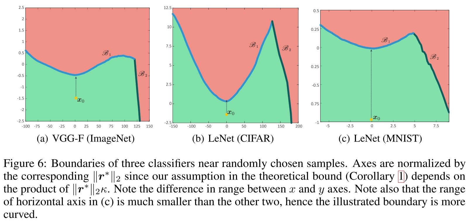
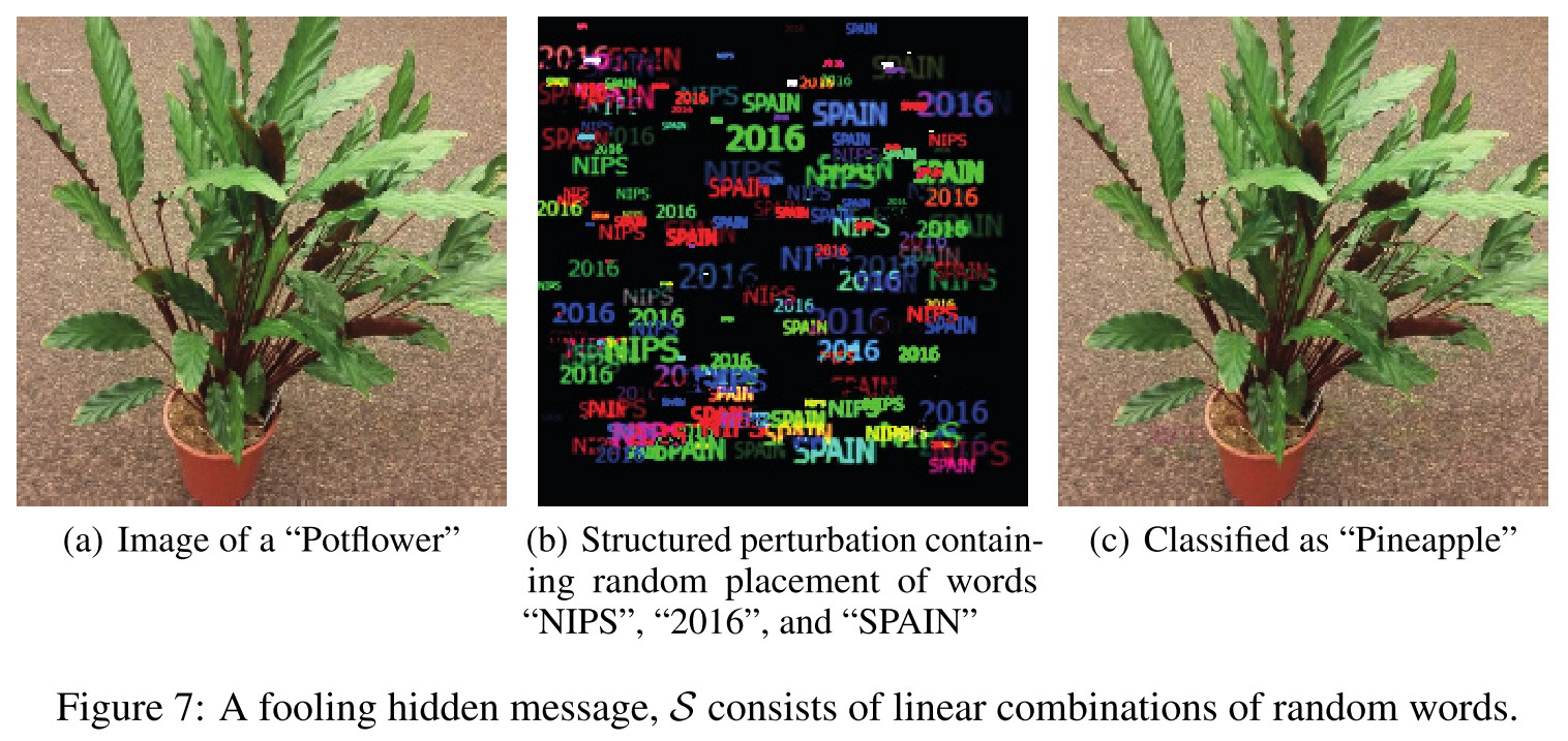
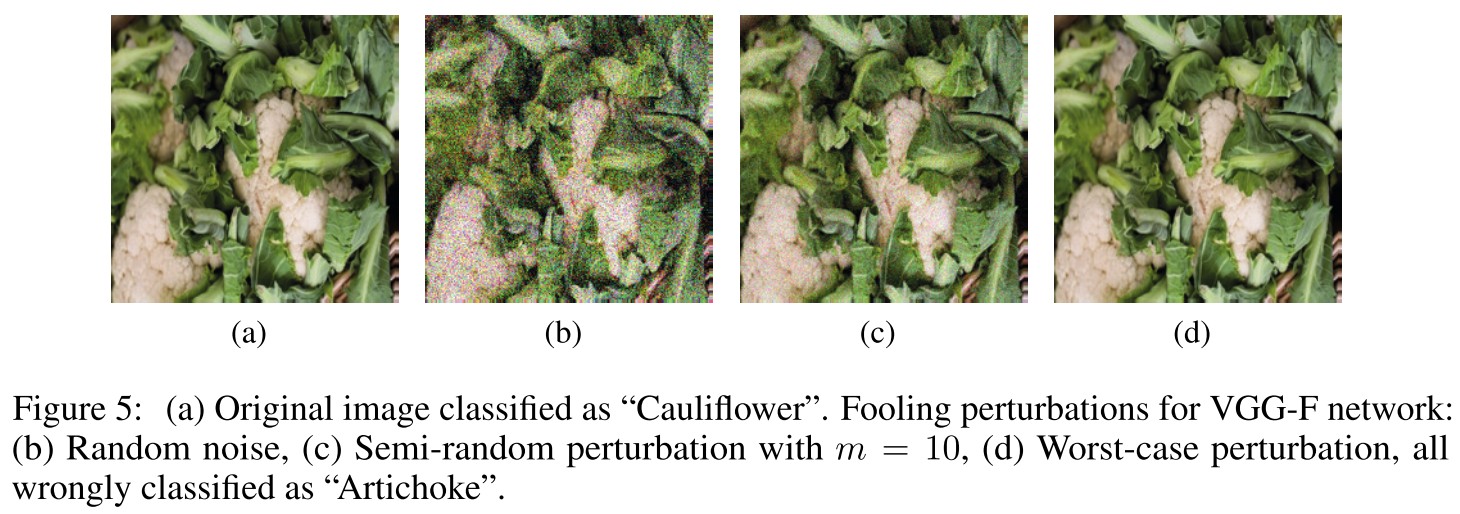
This shows that imperceptibly small structured messages can be added to an image causing data misclassification.

Conclusion

Our results show, in particular, that when the decision boundary has a small curvature, classifiers are robust to random noise in high dimensional classification problems (even if the robustness to adversarial perturbations is relatively small).

Moreover, for semi-random noise that is mostly random and only mildly adversarial (i.e., the subspace dimension is small), our results show that state-of-the-art classifiers remain vulnerable to such perturbations.

To improve the robustness to semi-random noise, our analysis encourages to impose geometric constraints on the curvature of the decision boundary, as we have shown the existence of an intimate relation between the robustness of classifiers and the curvature of the decision boundary.

Robustness of classifiers to universal perturbations - ICLR 2018

Paper: https://openreview.net/forum?id=ByrZyglCb

Seyed-Mohsen Moosavi-Dezfooli, Alhussein Fawzi, Omar Fawzi, Pascal Frossard, Stefano Soatto. Robustness of Classifiers to Universal Perturbations: A Geometric Perspective. ICLR 2018.

Adversarial vulnerability for any classifier - NIPS 2018

Paper: http://papers.nips.cc/paper/7394-adversarial-vulnerability-for-any-classifier

Alhussein Fawzi, Hamza Fawzi, Omar Fawzi. Adversarial vulnerability for any classifier. NIPS 2018.

In this paper, we study the phenomenon of adversarial perturbations under the assumption that the data is generated with a smooth generative model. We derive fundamental upper bounds on the robustness to perturbations of any classification function, and prove the existence of adversarial perturbations that transfer well across different classifiers with small risk.

For details, see Adversarial Vulnerability.

Inspirations

From the general idea, this paper suggests the following potentials

• Higher-dimensional data and more classes introduce less robustness.
• Unconstrained robustness (general robustness) can be increased by increasing in-distribution robustness (It seems to suggest that an accurate model is also important in terms of robustness?)
• A classifier is more robust if the boundary in latent space is more linear.

Adversarially robust generalization requires more data - NIPS 2018

Ludwig Schmidt, Shibani Santurkar, Dimitris Tsipras, Kunal Talwar, Aleksander Madry. Adversarially Robust Generalization Requires More Data. NIPS 2018. arXiv:1804.11285

We show that already in a simple natural data model, the sample complexity of robust learning can be significantly larger than that of “standard” learning.

As hinted in the title, they show that adversarially robust generalization requires more data. They address the following question:

How does the sample complexity of standard generalization compare to that of adversarially robust generalization?

Put differently, we ask if a dataset that allows for learning a good classifier also suffices for learning a robust one.

Overfitting in CIFAR-10

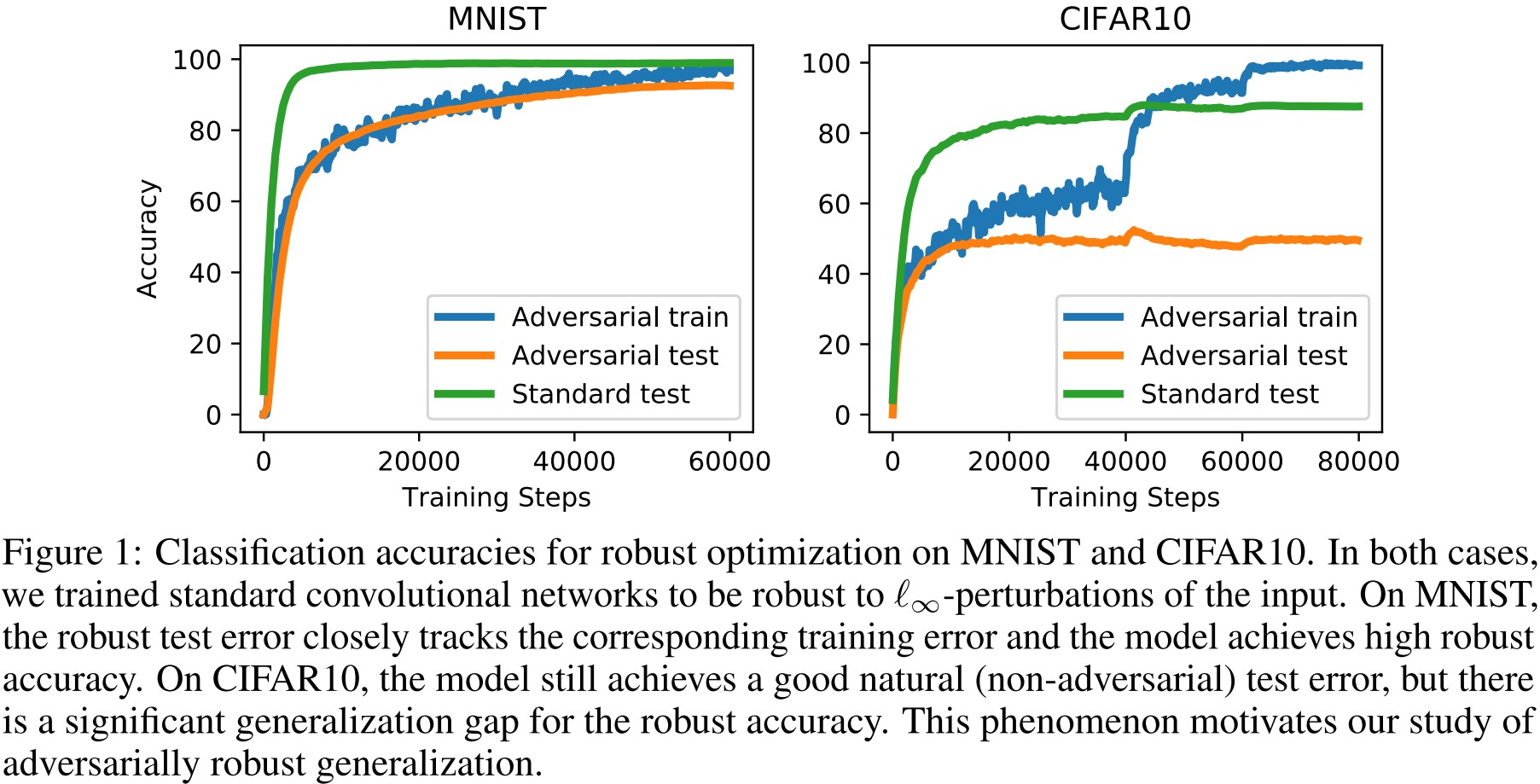
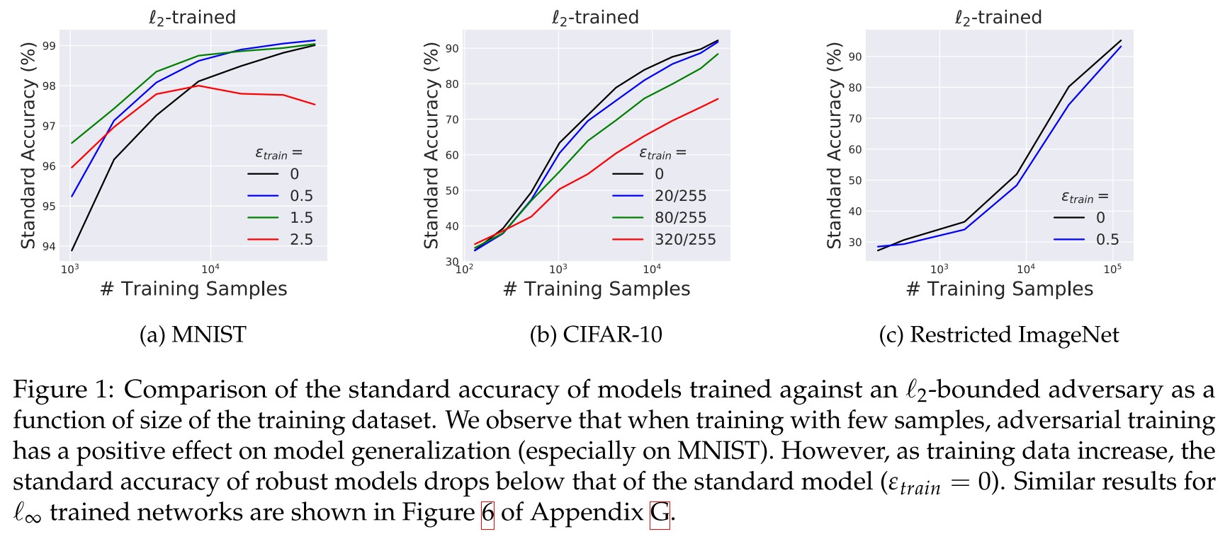
However, CIFAR10 offers a different picture. Here, the model (a wide residual network [61]) is still able to fully fit the training set even against an adversary, but the generalization gap is significantly larger.

As shown in Figure 1, on MNIST, adversarial training can achieve both high robust accuracy in training and test set while on CIFAR-10, there appears overfitting in adversarial accuracy.

Gaussian model

The Gaussian model is acquired by the following steps:

Let $\theta^*\in\R^d$ be the per-class mean vector and let $\sigma>0$ be the variance parameter. Then the $(\theta^*,\sigma)$-Gaussian model is defined by the following distribution over $(x,y)\in\R^d\times\{+1,-1\}$.

• First, draw a label $y\in\{+1,-1\}$ uniformly at random.
• Then sample the data point $x\in\R^d$ from $\mathcal{N}(y\cdot\theta^*,\sigma^2I)$.

The norm of the vector $\theta^*$ they use is approximately $\sqrt{d}$, leaving the main free parameter for controlling difficulty of the classification task is the variance $\sigma^2$, which controls the amount of overlap between the two classes.

The Classification error is defined as:

Let $\mathcal{P}:\R^d\times\{+1,-1\}\to\R$ be a distribution. Then the classification error $\beta$ of a classifier $f:\R^d\to\{+1,-1\}$ is defined as

The Robust classification error is defined as:

Let $\mathcal{P}:\R^d\times\{+1,-1\}\to\R$ be a distribution and let $\mathcal{B}:\R^d\to\mathscr{P}(\R^d)$ be a perturbation set. The the $\mathcal{B}$-robust classification error $\beta$ of a classifier $f:\R^d\to\{+1,-1\}$ is defined as

They focus on $\ell_{\infty}$-robustness, i.e.

Using a linear classifier defined as:

They prove the following theorem:

Theorem 4 Let $(x,y)$ be drawn from a $(\theta^*,\sigma)$-Gaussian model with $||\theta^*||_2=\sqrt{d}$ and $\sigma\le c\cdot d^{1/4}$, where $c$ is a universal constant. Let $\hat{w}\in\R^d$ be the vector $\hat{w}=y\cdot x$. Then with high probability, the linear classifier $f_{\hat{w}}$ has classification error at most 1%.

To minimize the number of parameters in our bounds, we have set the error probability to 1%.

This theorem states that as long as the variance is small enough, a simple linear classifier they consider can perform very well.

In terms of robust classification error, they show that achieving a low $\ell_{\infty}$-robust classification error requires significantly more samples.

Theorem 5 Let $(x_1,y_1),\dots,(x_n,y_n)$ be drawn i.i.d. from a $(\theta^*,\sigma)$-Gaussian model with $||\theta^*||_2=\sqrt{d}$ and $\sigma\le c_1\cdot d^{1/4}$. Let $\hat{w}\in\R^d$ be the weighted mean vector $\hat{w}=\frac{1}{n}\sum_{i=1}^n y_i x_i$. Then with high probability, the linear classifier $f_{\hat{w}}$ has $\ell_{\infty}^{\epsilon}$-robust classification error at most 1% if

where $c_1$ and $c_2$ are two universal constants.

Overall, the theorem shows that it is possible to learn an $\ell_{\infty}^\epsilon$-robust classifier in the Gaussian model as long as $\epsilon$ is bounded by a small constant and we have a large number of samples.

Theorem 6 Let $g_n$ be any learning algorithm, i.e. a function from $n$ samples to a binary classifier $f_n$. Moreover, let $\sigma=c_1\cdot d^{1/4}$, let $\epsilon\ge 0$, and let $\theta\in\R^d$ be drawn from $\mathcal{N}(0,I)$. We also draw $n$ samples from the $(\theta,\sigma)$-Gaussian model. Then the expected $\ell_{\infty}^\epsilon$-robust classification error of $f_n$ is at least $(1-1/d)\frac{1}{2}$ (typo?) if

Comparing Theorem 5 and Theorem 6, the sample complexity $n$ required for robust generalization is bounded as

This shows that for high-dimensional problems, adversarial robustness can provably require a significantly larger number of samples.

As a result, the lower bound provides transferable adversarial examples and applies to worst-case distribution shifts without a classifier-adaptive adversary.

Bernoulli model

When sampling a datapoint for a given class, we flip each bit of the corresponding class vertex with a certain probability. This data model is inspired by the MNIST dataset because MNIST images are close to binary (many pixels are almost fully black or white).

The Bernoulli model is acquired as follows

Let $\theta^*\in\{+1,-1\}^d$ bet the per-class mean vector and let $\tau >0$ be the class bias parameter. Then the $(\theta^*,\tau)$-Bernoulli model is defined by the following distribution over $(x,y)\in\{+1,-1\}^d\times\{+1,-1\}$:

• First, draw a label $y\in\{+1,-1\}$ uniformly at random from its domain.

• Then sample the data point $x\in\{+1,-1\}^d$ by sampling each coordinate $x_i$ from the distribution

  $$x_i=\begin{cases} y\cdot \theta^*_i&\text{ with probability }1/2+\tau\\ -y\cdot\theta^*_i&\text{ with probability }1/2-\tau \end{cases}$$

A smaller value of $\tau$ makes the samples less correlated with their respective class vectors, leading to a harder classification problem.

This model is similar to that of MNIST, since most pixels in a sample of MNIST are either near 0 or near 1.

Similarly, in standard generalization, there is

Theorem 8 Let $(x,y)$ be drawn from a $(\theta^*,\tau)$-Bernoulli model with $\tau\ge c\cdot d^{-1/4}$ where $c$ is a universal constant. Let $\hat{w}\in\R^d$ be the vector $\hat{w}=y\cdot x$. Then with high probability, the linear classifier $f_{\hat{w}}$ has classification error at most 1%.

As well as in robust generalization, there is

Theorem 9 Let $g_n$ be a linear classifier learning algorithm, i.e. a function from $n$ samples to a linear classifier $f_n$. Suppose that we choose $\theta^*$ uniformly from $\{+1,-1\}^d$ and draw $n$ samples from the $(\theta^*,\tau)$-Bernoulli model with $\tau=c_1\cdot d^{-1/4}$. Moreover, let $\epsilon<3\tau$ and $0<\gamma<1/2$. Then the expected $\ell_{\infty}^\epsilon$-robust classification error of $f_n$ is at least $\frac{1}{2}-\gamma$ if

They then show that non-linear classifiers can achieve a significantly improved robustness in this setting.

Consider the following thresholding operation $T:\R^d\to\R^d$ which is defined element-wise as

For $\epsilon< 1$, the thresholding operator undoes the action of any $\ell_{\infty}$-bounded adversary, i.e. $T(\mathcal{B}_{\infty}^\epsilon(x))=\{x\},\forall x\in\{+1,-1\}^d$.

Hence the following theorem:

Theorem 10 Let $(x,y)$ be drawn from a $(\theta^*,\tau)$-Bernoulli model with $\tau\ge c\cdot d^{-1/4}$ where $c$ is a universal constant. Let $\hat{w}\in\R^d$ bet the vector $\hat{w}=yx$. Then with high probability, the classifier $f_{\hat{w}}\circ T$ has $\ell_{\infty}^\epsilon$-robust classification error at most 1% for any $\epsilon<1$.

A binarization can defend well in this setting.

This discrepancy provides evidence that robust generalization requires a more nuanced understanding of the data distribution than standard generalization.

Experiments

We consider standard convolutional neural networks and train models on datasets of varying complexity. Specifically, we study the MNIST [34], CIFAR-10 [33], and SVHN [40] datasets.

We use a simple convolutional architecture for MNIST, a standard ResNet model [23] for CIFAR-10, and a wider ResNet [61] for SVHN.

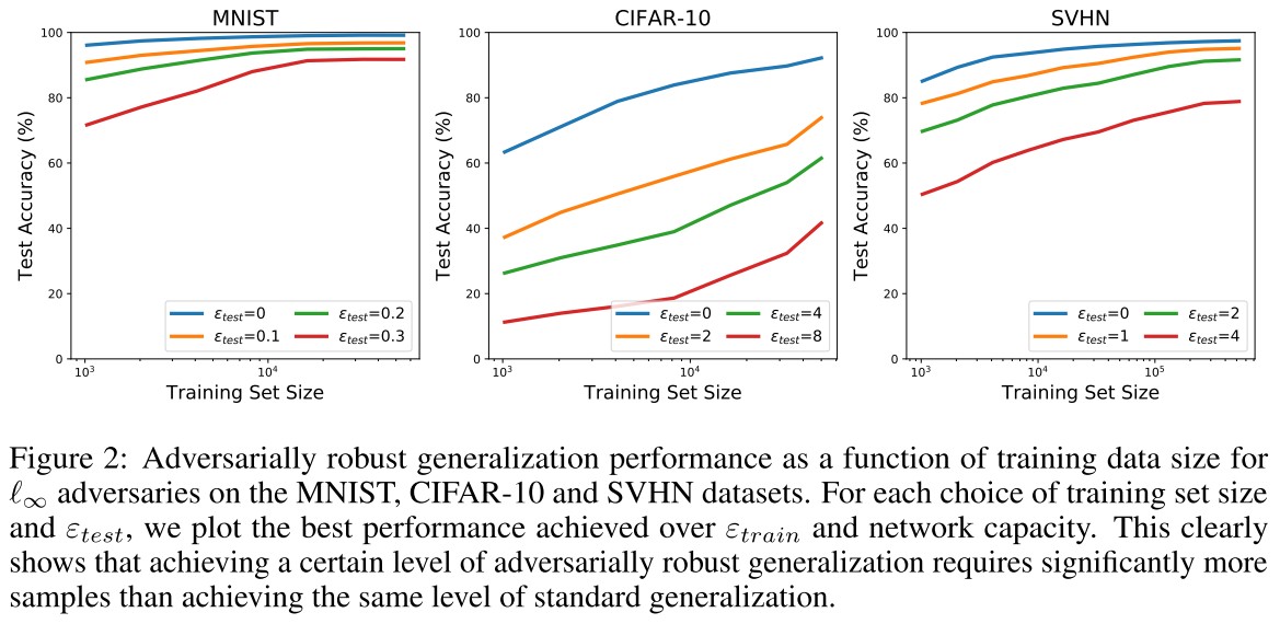
The plots demonstrate the need for more data to achieve adversarially robust generalization. For any fixed test set accuracy, the number of samples needed is significantly higher for robust generalization.

They also investigate whether thresholding can also improve the sample complexity of robust generalization against an $\ell_{\infty}$-adversary on MNIST.

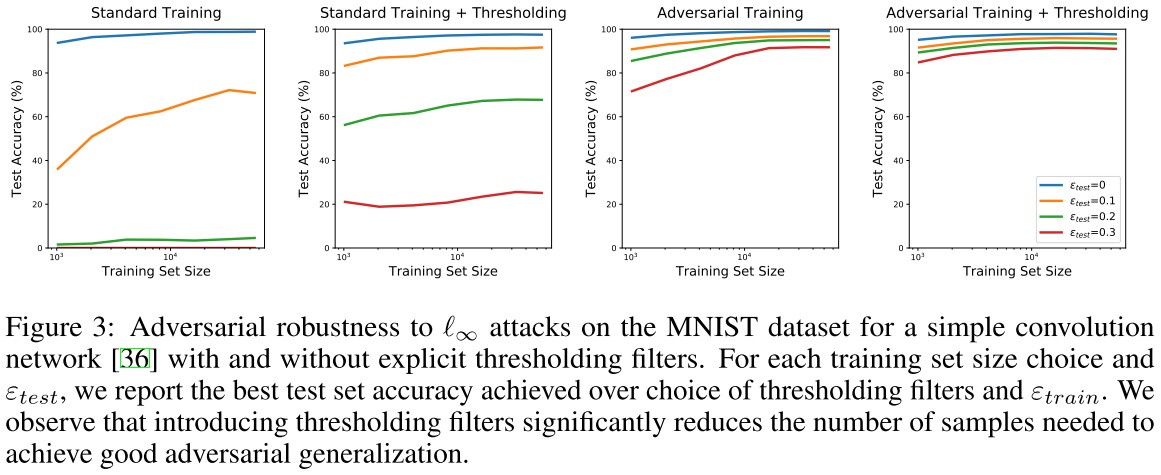
They replace the first convolutional layer with a fixed thresholding layer consisting of two channels, $ReLU(x-\epsilon_{filter})$ and $ReLU(1-x-\epsilon_{filter})$.

As predicted by our theory, the networks achieve good adversarially robust generalization with significantly fewer samples when thresholding filters are added.

It is also worth noting that the thresholding filters could have been learned by the original network architecture, and that this modification only decreases the capacity of the model.

Our findings emphasize network architecture as a crucial factor for learning adversarially robust networks from a limited number of samples.

We also experimented with thresholding filters on the CIFAR10 dataset, but did not observe any significant difference from the standard architecture.

Inspirations

Theoretically and empirically, this paper demonstrates that robust generalization requires more data, and by the way show the difference between MNIST and CIFAR-10.

It's interesting that a simple thresholding can improve the robustness of classifier on MNIST. Although they fail to do the same on CIFAR-10, I think it's worth further exploration.

Robustness May Be at Odds with Accuracy - ICLR 2019

Dimitris Tsipras, Shibani Santurkar, Logan Engstrom, Alexander Turner, Aleksander Madry. Robustness May Be at Odds with Accuracy. ICLR 2019. arXiv:1805.12152

Specifically, training robust models may not only be more resource-consuming, but also lead to a reduction of standard accuracy.

The representations learned by robust models tend to align better with salient data characteristics and human perception.

They try to answer the following question:

Why does there seem to be a trade-off between standard and adversarially robust accuracy?

The price of adversarial robustness

In canonical classification setting, the goal is to train models that have low expected loss (also known as population risk):

For adversarial robustness, the goal is to train models with low expected adversarial loss:

In which, $\Delta$ denotes the set of perturbations that th adversary can apply to induce misclassification. (In this paper, they focus on $l_p$-bounded perturbations, i.e. $\Delta=\{\delta\in\R^d|||\delta||_p\le\varepsilon\}$).

Adversarial training incorporates the two goals above, and aims at the following problem:

However, the robustness comes with a drop in accuracy and an increase in the training time.

Our point of start is a popular view of adversarial training as the “ultimate” form of data augmentation.

Thus, finding the worst-case $\delta$ corresponds to augmenting the training data in the “most confusing” and thus also “most helpful” manner.

But as shown in experiments, in most cases, adversarial training has a side effect to standard accuracy.

Adversarial robustness may be incompatible with standard accuracy

They construct the following dataset of input-label pairs $(x,y)$ sampled from a distribution $\mathcal{D}$

In which, $\mathcal{N}(\mu,\sigma^2)$ is a normal distribution with mean $\mu$ and variance $\sigma^2$, and $p\ge 0.5$. They chose $\eta$ to be large enough (e.g. $\eta=\Theta(1/\sqrt{d})$) such that a simple classifier attains high standard accuracy (>99%).

The parameter $p$ quantifies how correlated the feature $x_1$ is with the label. (They set $p=0.95$ for simplicity).

In short, they construct a dataset of two high dimensional Gaussian spheres but with one dimension correlated with the label.

A standard classification of the dataset is easy, e.g. a natural linear classifier

can achieve standard accuracy close to 100% for a large enough $d$.

The accuracy, i.e.

is >99% when $\eta\ge 3/\sqrt{d}$.

The standard classifier can utilize any feature that is even slightly correlated with the label.

But for adversarially trained model, this analogy breaks.

For instance, if $\varepsilon=2\eta$, an adversary can shift each weakly-correlated feature towards $-y$.

The classifier would now see a perturbed input $x^{'}$ such that each of the features $x^{'}_2,\dots,x_{d+1}^{'}$ are sampled i.i.d. from $\mathcal{N}(-\eta y,1)$.

Now, the accuracy achieved based on adversarial perturbed features is no better than 1% (reversed):

Intriguingly, this discussion draws a distinction between robust features ($x_1$) and non-robust features ($x_2,\dots,x_{d+1}$) that arises in the adversarial setting.

Theorem 2.1 (Robustness-accuracy trade-off). Any classifier that attains at least $1-\delta$ standard accuracy on $\mathcal{D}$ has robust accuracy at most $\frac{p}{1-p}\delta$ against an $l_{\infty}$-bounded adversary with $\varepsilon\ge2\eta$.

In short, a very strong adversary used in adversarial training will poison the accuracy.

Here, the trade-off between standard and adversarial accuracy is an inherent trait of the data distribution itself and not due to having insufficient samples.

Note, however, that humans can have lower accuracy in certain benchmarks compared to ML models (Karpathy, 2011, 2014; He et al., 2015; Gastaldi, 2017) potentially because ML models rely on brittle features that humans themselves are naturally invariant to.

The importance of adversarial training

Theorem 2.2 (Adversarial training matters). For $\eta\ge 4/\sqrt{d}$ and $p\le 0.975$ (the first feature is not perfect), a soft-margin SVM classifier of unit weight norm minimizing the distributional loss achieves a standard accuracy of $>99\%$ and adversarial accuracy of $<1\%$ against an $l_{\infty}$-bounded adversary of $\varepsilon\ge 2\eta$. Minimizing the distributional adversarial loss instead leads to a robust classifier that has standard and adversarial accuracy of $p$ against any $\varepsilon<1$.

This theorem shows that if our focus is on robust models, adversarial training is necessary to achieve non-trivial adversarial accuracy in this setting.

An interesting implication of our analysis is that standard training produces classifiers that rely on features that are weakly correlated with the correct label. (leading to the transferability of adversarial examples)

Further, we find that it is possible to obtain a robust classifier by directly training a standard model using only features that are relatively well-correlated with the label (without adversarial training).

Unexpected benefits of adversarial training

A model that achieves small loss for all perturbations in the set ∆, will necessarily have learned representations that are invariant to such perturbations. Thus, robust training can be viewed as a method to embed certain invariances in a model.

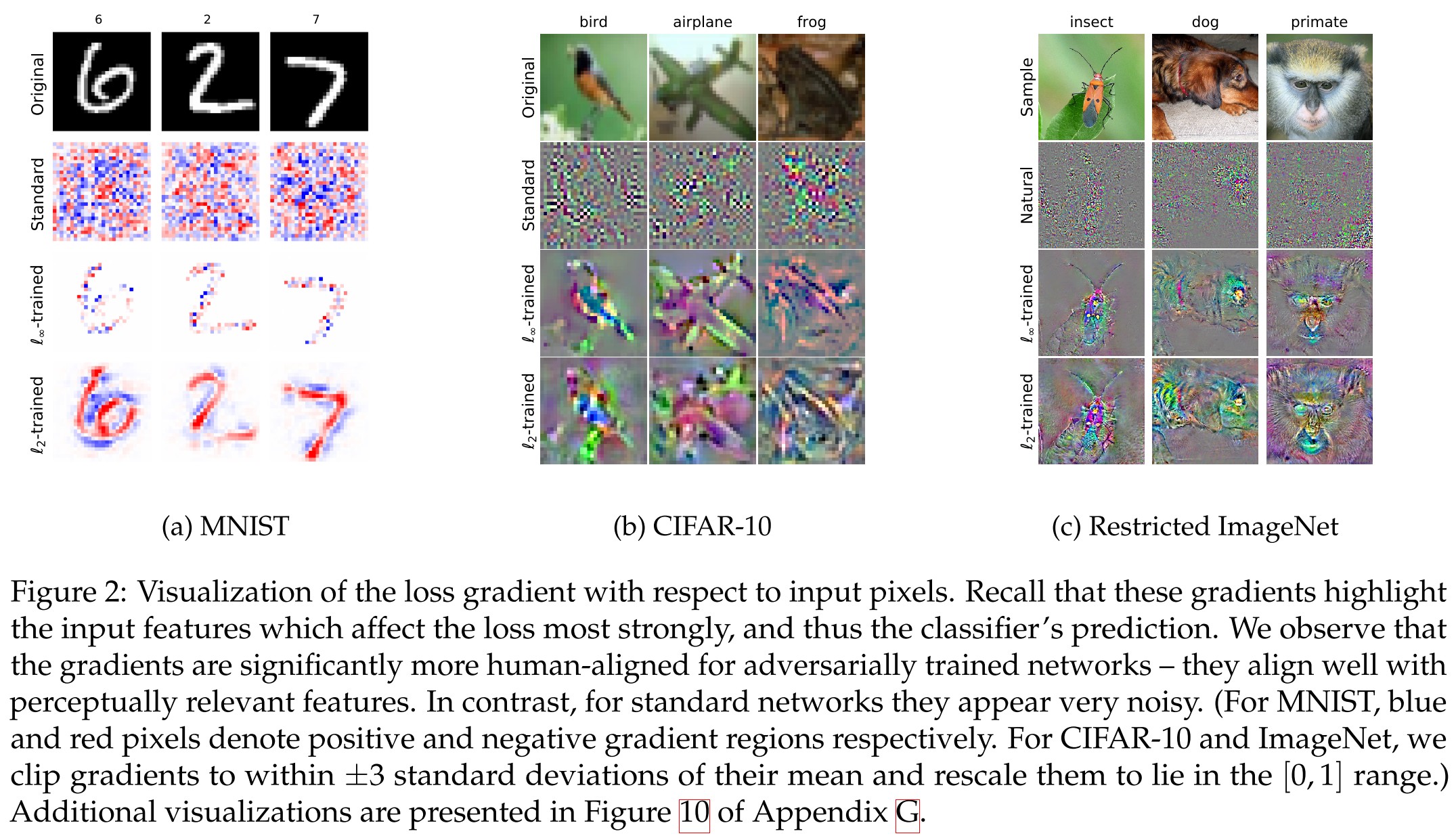
The adversarially trained model has a loss gradient better aligned with human perceptron.

By encoding the correct prior into the set of perturbations $\Delta$, adversarial training alone might be sufficient to yield more human-aligned gradients.

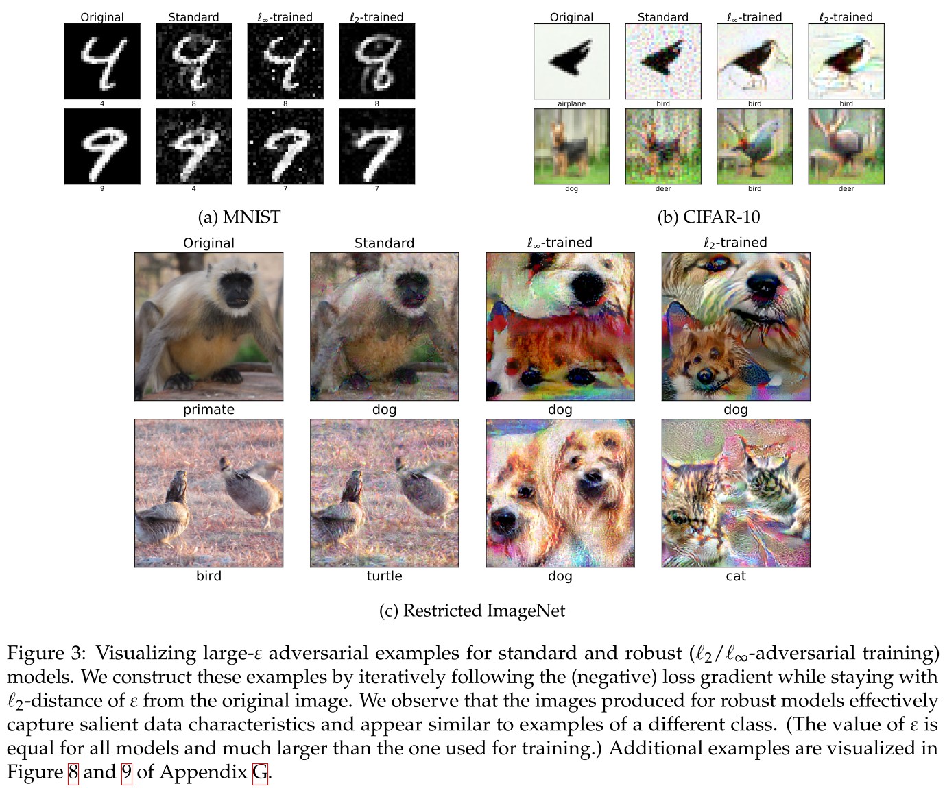
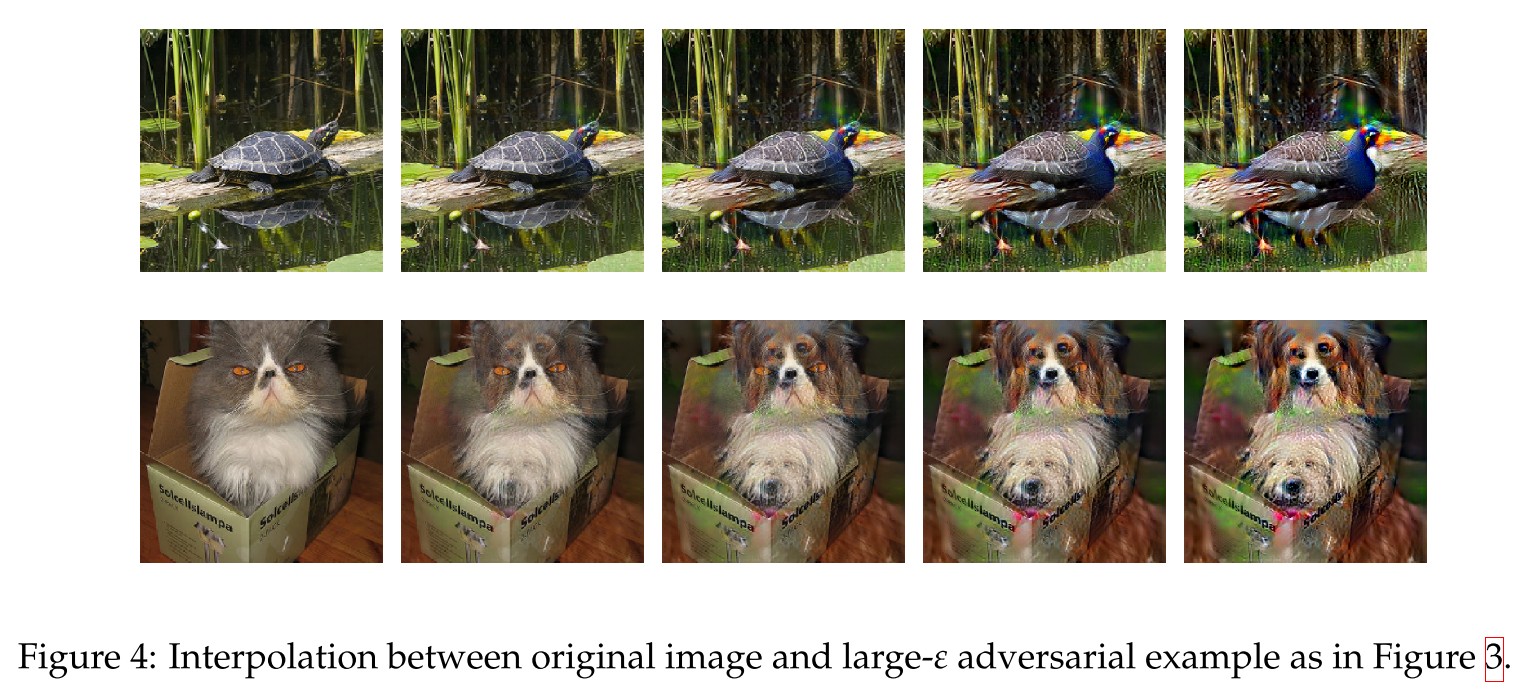
The adversarial examples generated for robust models appear to exhibit salient data charateristics. And consiquently

By linearly interpolating between the original image and the image produced by PGD we can produce a smooth, “perceptually plausible” interpolation between classes (Figure 4) .

Inspirations

This is truly a fruitful paper, theoretically, it points out the relation between robustness and accuracy, and empirically, it points out the better gradients manifested by robust models. Based on this paper, there are several directions for potential exploratories:

• Since the gradients are more interpretable, can one regularize the gradients to substitute adversarial training? (It has been achieved by JARN).
• Is it possible to use adversarially trained model it manipulate images instead of GAN?
• Based on Theorem 2.1, it seems that if $p=1-\delta$, one can get an equally robust and accurate model. And $p\ge0.5$ for the theorem to stand, thus the model is equally robust and accurate with accuracy of 50%. It seems to coincide the reported robustness accuracy of C&W attack.
• Based on Theorem 2.1, a very strong adversary, i.e. $\varepsilon\ge 2\eta$ will tamper the accuracy when involved in adversarial training, it seem that one can improve adversarial training by restricting the ability of adversary involved. (It has been done partially be Friendly Adversarial Training)

Cause of Adversarial Example

Adversarial spheres - 2018

Justin Gilmer, Luke Metz, Fartash Faghri, Samuel S. Schoenholz, Maithra Raghu, Martin Wattenberg, Ian Goodfellow. The Relationship Between High-Dimensional Geometry and Adversarial Examples. 2018. arXiv:1801.02774v3

We hypothesize that this counterintuitive behavior is a result of the high-dimensional geometry of the data manifold, and explore this hypothesis on a simple high-dimensional dataset.

Adversarial examples are not bugs, they are features - NIPS 2019

Andrew Ilyas, Shibani Santurkar, Dimitris Tsipras, Logan Engstrom, Brandon Tran, and Aleksander Madry. Adversarial examples are not bugs, they are features. In Advances in Neural Information Processing Systems, pages 125–136, 2019. arXiv:1905.02175v3

They claim that

Adversarial vulnerability is a direct result of our models’ sensitivity to well-generalizing features in the data.

In fact, we find that standard ML datasets do admit highly predictive yet imperceptible features.

Since any two models are likely to learn similar non-robust features, perturbations that manipulate such features will apply to both.

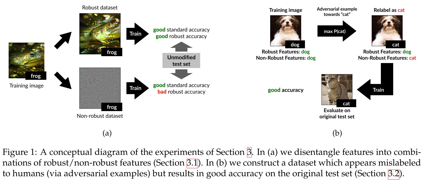
To corroborate their claim, they designed two training dataset to show that it's possible to disentangle robust and non-robust features from the standard image classification dataset.

Definitions

They consider a binary classification scenario.

The input-label pairs $(x,y)\in\cal{X}\times\{\pm 1\}$ are sampled from a distribution $\cal{D}$, and the goal is to learn a classifier $C:\cal{X}\to\{\pm 1\}$ which predicts a label $y$ corresponding to a given input $x$.

The feature is defined as a function mapping from the input space $\cal{X}$ to the real numbers, i.e. the set of all features is $\mathcal{F}=\{f:\mathcal{X}\to\Bbb{R}\}$, for the simplicity for analysis, they assume that $\Bbb{E}_{(x,y)\sim\mathcal{D}}[f(x)]=0$ and $\Bbb{E}_{(x,y)\sim\mathcal{D}}[f(x)^2]=1$.

The features are categorized in the following manner:

• $\rho$-useful features

  For a given distribution $\cal{D}$, a feature is called $f$ $\rho$-useful ($\rho>0$) if it is correlated with the true label in experience, i.e.

  $$\Bbb{E}_{(x,y)\sim\mathcal{D}}[y\cdot f(x)]\ge \rho$$

  The largest $\rho$ for which feature $f$ is $\rho$-useful under distribution $\cal{D}$ is denoted as $\rho_{\cal{D}}(f)$.

• $\gamma$-robustly useful features

  For a $\rho$-useful feature $f$, the feature is referred as a robust feature if $f$ remains $\gamma$-useful under adversarial perturbation $\delta\in \Delta(x)$, i.e.

  $$\Bbb{E}_{(x,y)\sim\cal{D}}\left[\inf_{\delta\in\Delta(x)}y\cdot f(x+\delta)\right]\ge \gamma$$

• Useful, non-robust features

  A useful, non-robust feature is a feature which is $\rho$-useful for some $\rho$ bounded away from zero, but is not a $\gamma$-robust feature for any $\gamma\ge 0$.

In short, a feature that still correlates with the corresponding label under permitted adversarial perturbations is defined as a robust feature here.

For a given input $x$, the classifier $C=(F,w,b)$ predicts the label $y$ as

The standard training is performed by minimizing a loss function, e.g.

As shown by the term, no distinction exists between robust and non-robust features in standard training, the only distinguishing factor of a feature is its $\rho$-usefulness.

The robust training involves an adversary making any useful but non-robust features anti-correlated with the true label, i.e.

The process can be viewed as explicitly preventing the classifier from learning a useful but non-robust combination of features.

Robust features

Given a robust (i.e. adversarially trained) model $C$ , the desired robust distribution $\hat{\cal{D}}_R$ should suffices

In which, $F_C$ denotes the features utilized by $C$.

They use an one-to-one mapping $x\mapsto x_r$ to construct a training set for $\hat{\cal{D}}_R$ by the following optimization:

In which, $g$ is the mapping from input $x$ to the representation layer.

To approximate the condition that $f\notin F_C$, which is not accessible, they choose the starting point of gradient descent for the optimization to be an input $x_0$ drawn from $\cal{D}$ independently of the label of $x$. ($f(x_0)\cdot y\simeq 0$)

Using the same procedure but with a non-robust model $C$, they crafted the training set for $\hat{\cal{D}}_{NR}$.

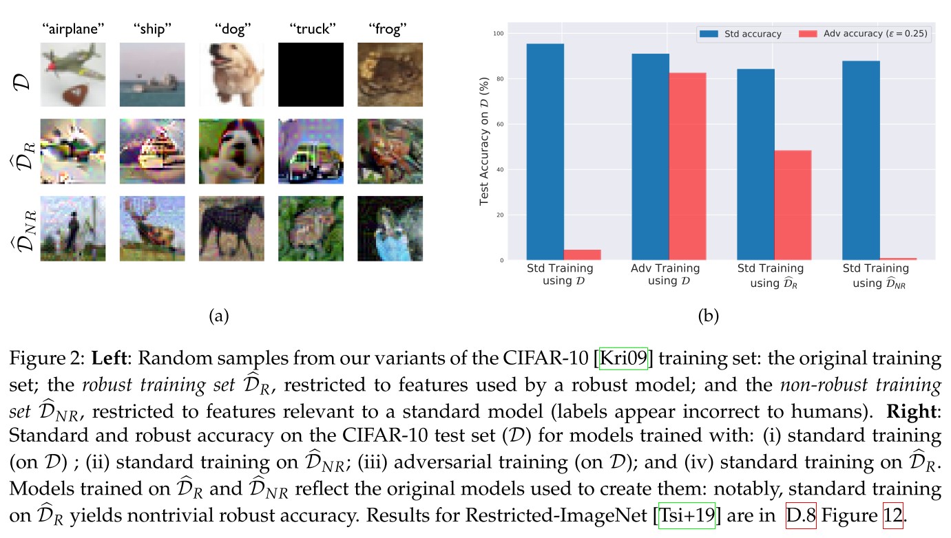
As shown by Figure 2

By filtering out non-robust features from the dataset (e.g. by restricting the set of available features to those used by a robust model), one can train a robust model using standard training.

Non-robust features

They constructed a dataset where only the non-robust features are useful for classification by adversarially perturbing the input $x$ in input-label pair $(x,y)$ such that the adversarial example $x_{adv}$ is classified as $t$, i.e.

They then use the resulting input-label pair $(x_{adv},t)$ to constructed the desired dataset of distribution $\hat{\cal{D}}_{rand}$ such that

In this dataset, all of the inputs labeled with class $t$ should have non-robust features correlated with $t$ but robust features correlated with the original class $y$.

When $t$ is chosen deterministically based on $y$, it yields a stronger version $\hat{\cal{D}}_{det}$ such that

Models trained on these dataset show a surprisingly generalization ability.

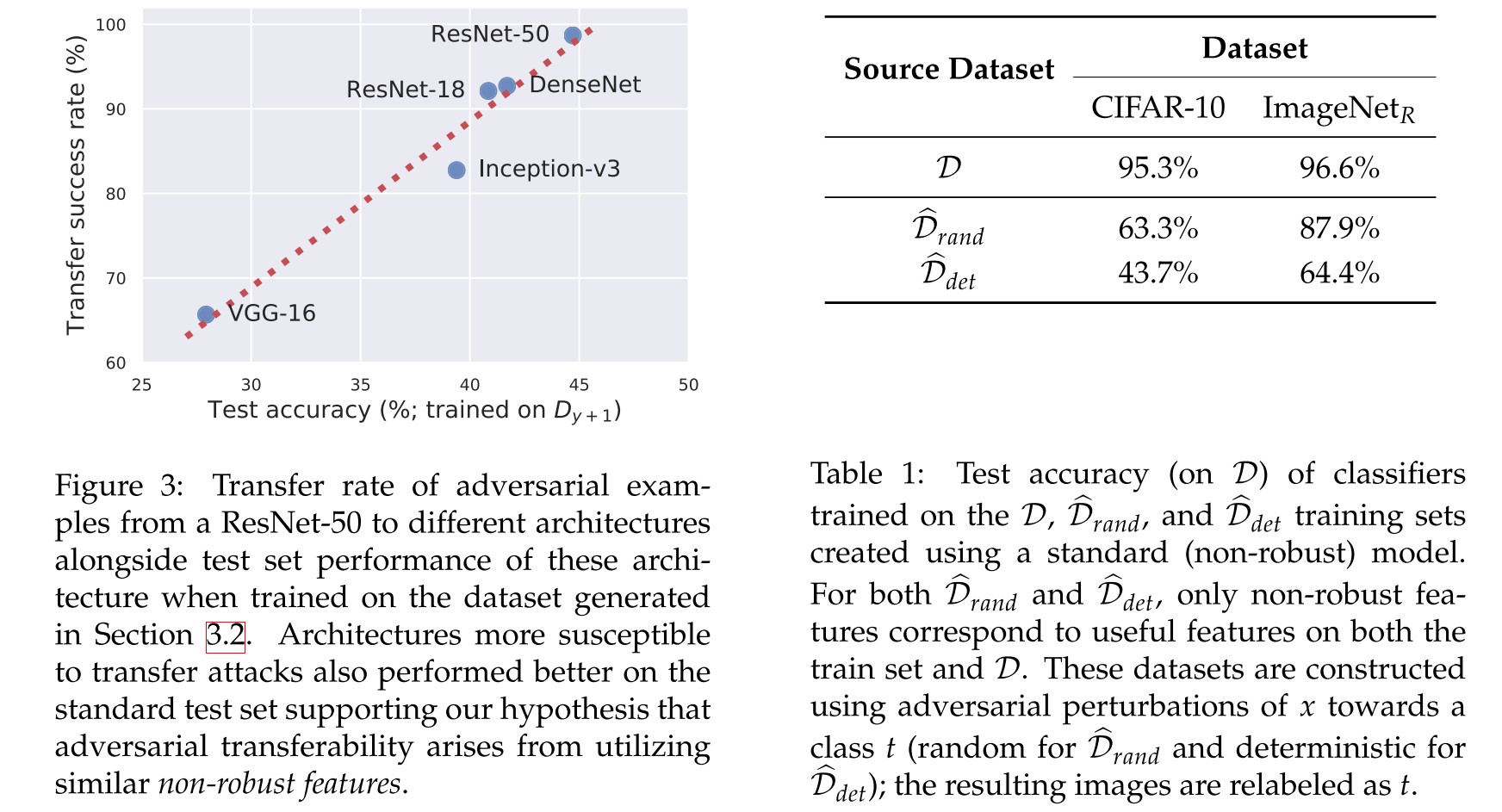
Given that such features are inherent to the data distribution, different classifiers trained on independent samples from that distribution are likely to utilize similar non-robust features. Consequently, an adversarial example constructed by exploiting the non-robust features learned by one classifier will transfer to any other classifier utilizing these features in a similar manner.

Theoretical framework

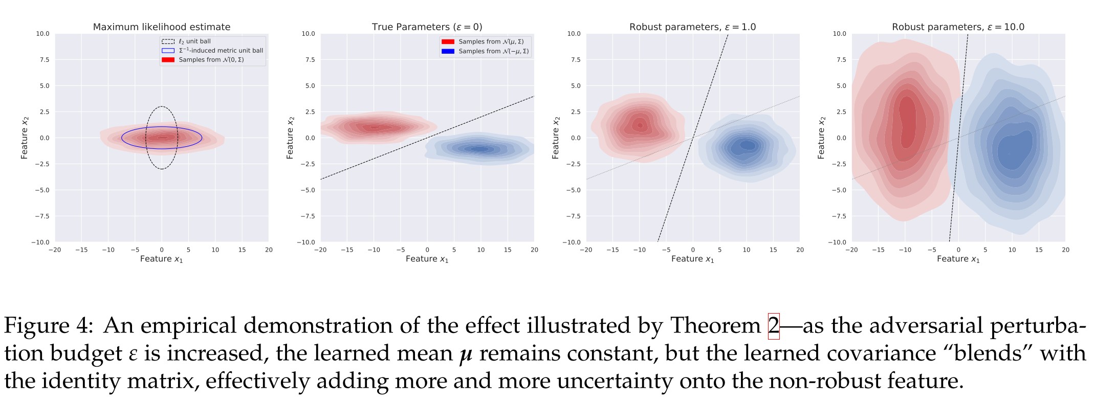
They study a simple problem of maximum likelihood classification between two Gaussian distributions.

Given samples $(x,y)$ sampled from $\cal{D}$ according to

The goal is to learn parameters $\Theta=(\mu,\Sigma)$ such that

In which, $l(x;\mu,\Sigma)$ represents the Gaussian negative log-likelihood (NLL) function, i.e. (?)

Intuitively, we find the parameters $\mu,\Sigma$ which maximize the likelihood of the sampled data under the given model.

The classification of this model is done with likelihood test, given an unlabeled sample $x$, the predicted $y$ is calculated by

The robust analogue of this problem (avdersarial training) is

Theorem 1 (Adversarial vulnerability from misalignment). Consider an adversary whose perturbation is determined by the "Lagrangian penalty" form, i.e.

where $C\ge \frac{1}{\sigma_{min}(\Sigma_*)}$ is a constant trading off NLL minimization and the adversarial constraint. Then, the adversarial loss $\cal{L}_{adv}$ incurred by the non-robustly learned $(\mu,\Sigma)$ is given by

and, for a fixed $tr(\Sigma_*)=k$ the above is minimized by $\Sigma_*=\frac{k}{d}I$.

Theorem 2 (Robustly learned parameters) Just as in the non-robust case, $\mu_r=\mu^*$,i.e. the true mean is learned. For the robust covariance $\Sigma_r$, there exists an $\varepsilon_0>0$, such that for any $\varepsilon\in[0,\varepsilon_0)$,

Theorem 3 (Gradient alignment) Let $f(x)$ and $f_r(x)$ be monotonic classifiers based on the linear separator induced by standard and $l_2$-bounded maximum likelihood classification, respectively. The maximum angle formed between the gradient of the classifier (w.r.t input) and the vector connecting the classes can be smaller for the robust model, i.e.

Our theoretical analysis suggests that rather than offering any quantitative classification benefits, a natural way to view the role of robust optimization is as enforcing a prior over the features learned by the classifier.

Inspirations

Based on the theorems proposed in this paper, it's possible that

• One can achieve adversarial robustness by filtering out the non-robust features in dataset.
• One can improve adversarial robustness by aligning the Jacobians with the inputs (It has been achieved by JARN).

Adversarial Examples Are a Natural Consequence of Test Error in Noise - ICML 2019

Nic Ford, Justin Gilmer, Nicolas Carlini, Dogus Cubuk. Adversarial Examples Are a Natural Consequence of Test Error in Noise. arXiv:1901.10513

This paper finds connection between adversarial robustness and corruption robustness and indicates that increasing adversarial robustness can also increase corruption robustness.

In this paper we provide both empirical and theoretical evidence that these are two manifestations of the same underlying phenomenon, establishing close connections between the adversarial robustness and corruption robustness research programs.

Based on our results we recommend that future adversarial defenses consider evaluating the robustness of their methods to distributional shift with benchmarks such as Imagenet-C.

Motivation

Several recent papers (Gilmer et al., 2018b; Mahloujifar et al., 2018; Dohmatob, 2018; Fawzi et al., 2018a) use concentration of measure to prove rigorous upper bounds on adversarial robustness for certain distributions in terms of test error, suggesting non-zero test error may imply the existence of adversarial perturbations. (i.e. $r_{unc}(f)\ge \frac{1}{2}r_{in}(x)$)

This may seem in contradiction with empirical observations that increasing small perturbation robustness tends to reduce model accuracy (Tsipras et al., 2018). (i.e. Adversarial Robustness May be at Odds with Accuracy.)

It could be the case that hard bounds on adversarial robustness in terms of test error exist, but current classifiers have yet to approach these hard bounds.

I do not think these two are contradictory, since the theorem in the latter is based on the scenario when the adversary is very strong (i.e. $\varepsilon=2\eta$).

Adversarial and corruption robustness

Given an error set of classifier $E$ (i.e. the set of data points that a classifier makes incorrect predictions), a natural distribution of image $p$, the two robustness is defined as

• corruption robustness

  Given a corrupted image distribution $q$, it's defined as

  $$\Bbb{P}_{x\sim q}[x\not\in E]$$

  It's the probability that a random sample from $q$ is not an error. (Higher is better.)

• adversarial robustness

  For a clean image $x$ and a metric on the input space $d$ (denote the distance from $x$ to its nearest point in $E$ as $d(x,E)$), it's defined as

  $$\Bbb{P}_{x\sim p}[d(x,E)>\epsilon]$$

  It's the probability that a random sample from $p$ is not within distance $\epsilon$ of some point in the error set.

  Higher is better. If a sample is within the $\epsilon$ distance of error set, it means that one can craft an adversarial example by moving this sample for a distance of $\epsilon$.

Errors in Gaussian noise suggest adversarial examples

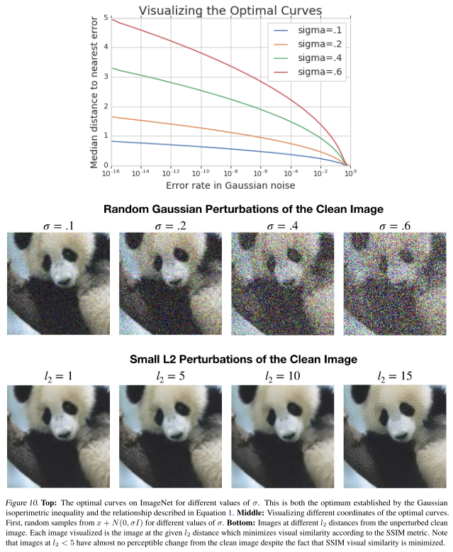
For linear models, the error rate in Gaussian noise exactly determines the distance to the decision boundary.

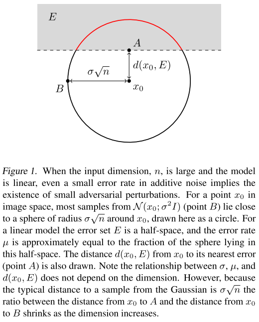
For a clean image $x_0$, consider the Gaussian distribution $\mathcal{N}(x_0;\sigma^2 I)$. For a fixed $\mu$, let $\sigma(x_0,\mu)$ be the $\sigma$ for which the error rate is $\mu$, i.e.

$\mu$ is the expectation of the probabilities that a $x$ sampled from $\mathcal{N}(x_0;\sigma^2 I)$ falls into the error set (crosses the boundary).

Consider the $l_2$ distance, i.e. $d=||\cdot||_2$, there is

In which,

is the cdf of the univariate standard normal distribution.

As the distance from a typical sample from $\mathcal{N}(x_0;\sigma^2I)$ to the center $x_0$ is $\sigma\sqrt{n}$, the distance to the decision boundary will be significantly smaller than the distance to a noisy image when the dimension $n$ is large.

This is a little confusing, since $\sigma\sqrt{n}$ is proportional to teh dimension. The $\mu$ is the proportion of the shaded area in the entire sphere, so, when the sphere goes into higher dimension, the shaded area will be closer to the center to maintain a fixed $\mu$.

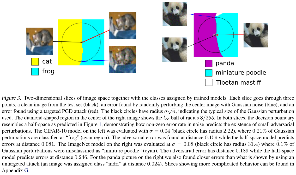
It indicates that even the error rate is ralatively small for random Gaussian perturbations, the feasible nearest perturbation is still very close to the original image, as shown in Figure 10.

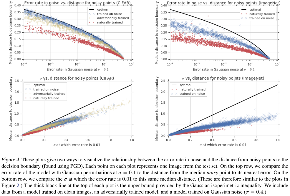
The neural network is of course not linear, so they investigate the ratio between $d(x_0,E)$ and $\sigma(x_0,\mu)$ for it. They examine this relationship on $\mu=0.01$ , and compare $\sigma(x_0,0.01)$ with $d(x_0,E)$, the latter is acquired using PGD.

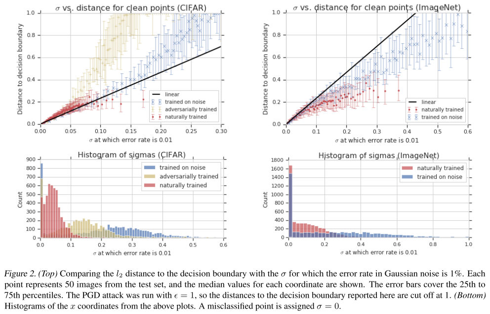
First, adversarial training and Gaussian data augmentation increased both $\sigma(x_0,0.01)$ and $d(x_0,E)$ on average.

While both augmentation methods do improve both quantities, Gaussian data augmentation had a greater effect on $\sigma$ (as seen in the histograms) while adversarial training had a greater effect on $d$.

They further draw two-dimensional slices in image space through three points to prove the correctness of half-space model.

Concentration of measure for noisy images

Denote the median distance from one of these noisy images in the neighbor of $x_0$ to the nearest error as $\epsilon^*_q(E)$.

It's the $\epsilon$ for which

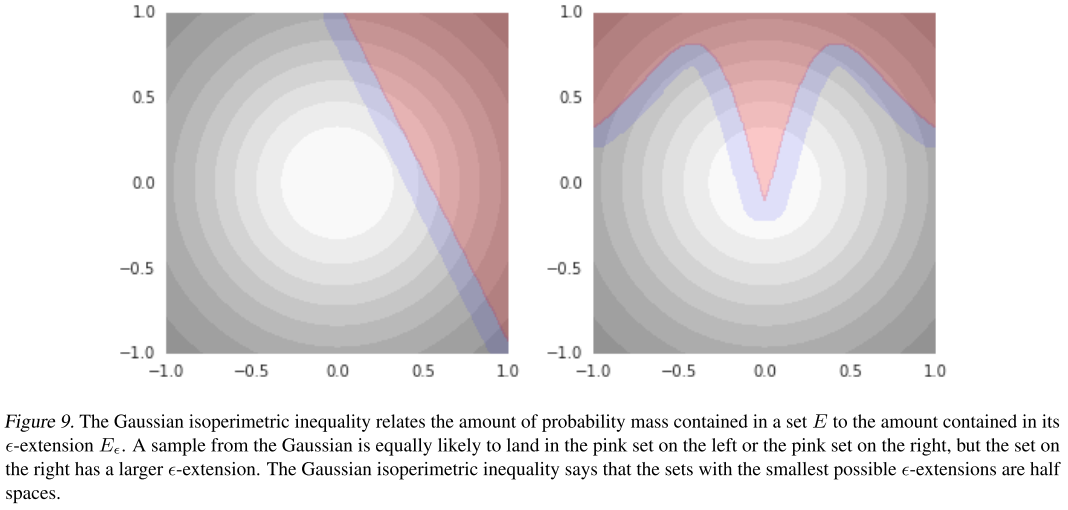
Theorem (Gaussian Isoperimetric Inequality). Let $q=\mathcal{N}(0;\sigma^2 I)$ be the Gaussian distribution on $\R^n$ with variance $\sigma^2I$, and, for some set $E\sube \R^n$, let $\mu=\Bbb{P}_{x\sim q}[x\in E]$. As before, write $\Phi$ for the cdf of the univariate standard normal distribution. if $\mu\ge\frac{1}{2}$, then $\epsilon^*_q(E)=0.$ Otherwise, $\epsilon^*_q(E)\le-\sigma\Phi^{-1}(\mu)$, with equality when $E$ is a half space.

So, among models with some fixed error rate $\Bbb{P}_{x\sim q}[x\in E]$, the most robust are the ones whose error set is a half space (as shown in Figure 1).

The sentence above is confusing. As shown in Figure 9, when the boundary is flat, the proportion of the purple area, i.e. the $\epsilon$-band of error sets reaches its minimum if the error rate, i.e. the proportion of the red area is fixed.

They further evaluate the theorem on CIFAR-10 and ImageNet test sets.

For each test image, we took 1,000 samples from the corresponding Gaussian and estimated $\epsilon^*_p$ using PGD with 200 steps one each sample and reported the median.

This shows that improved adversarial robustness results in improved robustness to large random perturbations, as the isoperimetric inequality says it must.

The adversarial training pushes the boundary behind and consequently reduces the proportion of the shaded area in Figure 1.

Evaluating corruption robustness

Gaussian data augmentation and adversarial training both improve the overall benchmark1, which requires averaging the performance across all corruptions, and the results were quite close.

Interestingly, both methods performed much worse than the clean model on the fog and contrast corruptions. (It's also reported on Fourier Perspective)

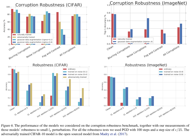
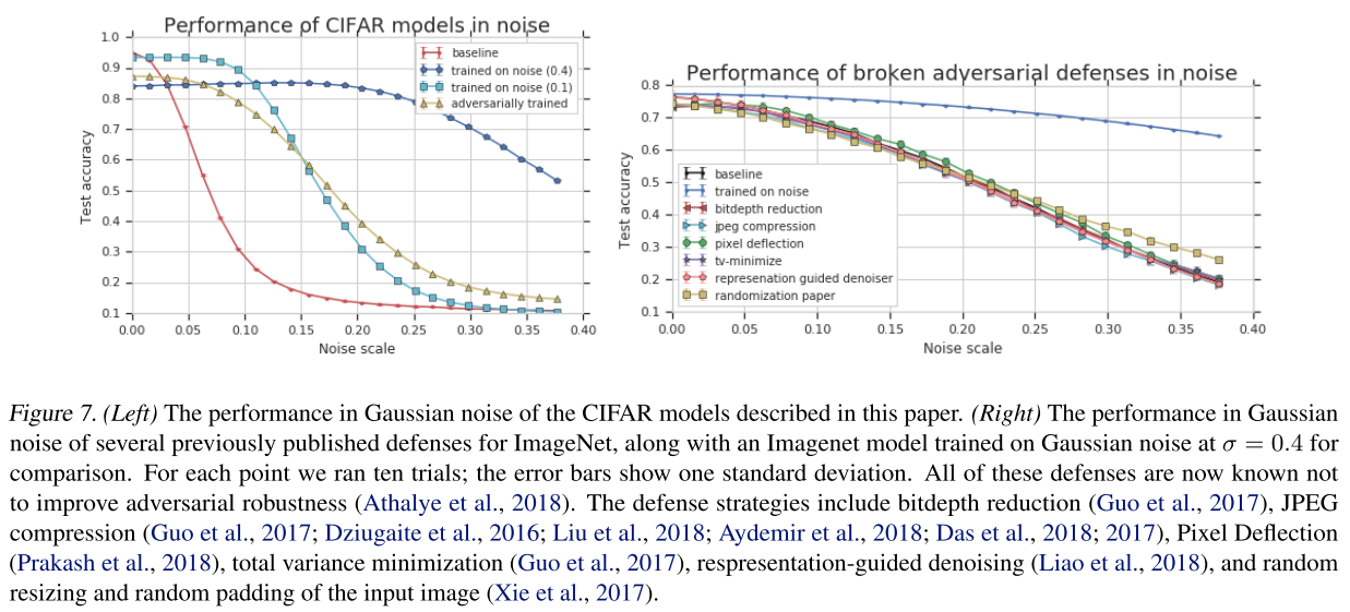
As shown in Figure 6, the Gaussian augmentation also helps with the adversarial robustness, although only a little. And as shown in Figure 7, they discover that those methods relying on gradient masking also fail to help with Gaussian noise.

Conclusion

The nearby errors we can find show up at the same distance scales we would expect from a linear model with the same corruption robustness.

Concentration of measure shows that a non-zero error rate in Gaussian noise logically implies the existence of small adversarial perturbations of noisy images.

Finally, training procedures designed to improve adversarial robustness also improve many types of corruption robustness, and training on Gaussian noise moderately improves adversarial robustness.

Inspirations

This is a fruitful paper. They build a bridge between the research of adversarial robustness and corruption robustness, and empirically show that the improvement of adversarial robustness also helps with the improvement of Gaussian noise corruption robustness.

Through the theorems they form, the purpose of these two robustness coincide with each other and they suggest further collaboration of these two communities of researchers.

They also demenstrate empirically that those defense methods reported to be relying on gradient masking also fail to help with Gaussian noise corruption, which is a new meter for defense methods to self evaluate.

The most amazing although not surprising is the result of the curse of dimensionality in robustness of model, i.e. a very small tolaratable error rate of Gaussian noise error entails the existence of very subtle adversarial perturbations.

It indicates that probably some noise augmentation can do the work for the heavy adversarial training.