Adversarial Example in Object Detection
By Haoyang Li, 2020.9.30 ~ 2020.10
Content
Adversarial Example in Object DetectionContentConceptsObject DetectionAdversarial ExampleTask DescriptionAttacksAdversarial glasses - SIGSAC 2016Threat modelProblem formulationPerformanceAgainst the Viola-Jones face detectorDAG - ICCV 2017Problem formulationDense Adversary GenerationPerformanceTransferabilityInspirationsRP2 -CVPR 2018Problem formulationStrategyPerformanceInspirationsAdversarial patch - CVPR workshop 2019StrategyLossPerformanceInspirationsAdversarial T-Shirt - ECCV 2020Problem definitionStrategyPatch applierThin Plate Spline mappingProblem formulationPerformanceInspirationsInvisibility cloak - ECCV 2020DefenseTowards Adversarially Robust Object Detection - ICCV 2019One-stage object detectorObservationAdversarial training for robust detectionPerformance
Concepts
Object Detection
A Simple Survey of Object Detection
Given an image, an object detection system predicts each object's location (x and y position), size (height and width), class (what it is) and confidence (how confident).
The modern methods based on training define the problem as follows. For a large set of input images , the human eyes will detect a set of objects for each input, the set of these set is denoted as . Each object is denoted by its location (generally four values ), class and confidence. The goal is to construct a system with tunable parameters to estimate the real human object detection system , such that , with a pre-defined prior generator for easier optimization:
The state-of-art object detection methods follow a paradigm of extracting features and tuning customized network heads. A typical structure is a cascade of backbone network (such as ResNet) and classifier/regressor head.
Most methods predict offsets relative to pre-defined priors (such as anchors, grids or dense centers), although some refreshing ideas are emerging. The very recent method, DETR, escapes from most priors and customized heads, while still trapped by a feature extractor.
Adversarial Example
the Landscape of Adversarial Example
Adversarial examples are such examples that 1) make no difference to human eyes 2) fool the targeted system to malfunction. Many methods in deep learning have been discovered to be vulnerable to adversarial examples, along with many methods to generate adversarial examples.
For a target system estimated from original map and a target input , the goal is to generate an adversarial example with a minimal perturbation , such that :
By the attacker's knowledge of the system, these methods are divided into white-box and black-box, the former assumes the attacker have full knowledge of the system while the latter does not make such assumptions, which makes the former easier and popular in literature, less meaningful in practice and the latter more difficult and weirder in literature, more meaningful in practice. Between black and white, some also call the scenario when attacker has limited knowledge as gray-box.
The problem of generating adversarial examples is a reversed optimization problem, in which the parameters of the targeted model is fixed, while the input is tuned to mislead the model under certain constraints. The white-box methods generally utilize the gradients of the model, and the black-box methods either utilize the transferability of adversarial examples, or solve the problem with zero-order optimization algorithms (e.g. evolutionary algorithms, reinforcement learning, etc. ).
Most white-box attack (i.e. the most prevailing methods) reforms the problem into a reversed training where the loss is maximized rather than minimized.
The defense of adversarial attack is more difficult and no method has defended all adversarial attacks. Theoretically, a min-max optimization is formulated with the idea of adversarial training to train a robust model.
The inner formulation searches an optimal perturbation in allowed perturbations and the outer formulation searches an optimal parameter to minimize the loss function respect to the perturbed example. However, even the model trained with adversarial training is not highly robust. The defense of adversarial attack is still an unsolved problem.
Task Description
An object detection system takes an image and predict the location, class and confidence for each object in image. The adversarial attack against it is a reversed task. Given a well-tuned object detection system and the task is to generate an image that's normal to human eyes while fooled the object detection system.
The non-targeted attack is to fool the system to overlook/mislocate/misclassify the target object (i.e. decrease the recall), or mistake the background as object (i.e. decrease the precision).
The targeted attack is to fool the system to mistake the target as another designated object or mistake the background as designated objects.
Goal:
- Stealthier (more inconspicuous to human eyes)
- Higher success rate (more threatening to system)
- Faster (more practical to attack)
Attacks
Adversarial glasses - SIGSAC 2016
Paper: https://www.cs.cmu.edu/~sbhagava/papers/face-rec-ccs16.pdf
Sharif, Mahmood & Bhagavatula, Sruti & Bauer, Lujo & Reiter, Michael. (2016). Accessorize to a Crime: Real and Stealthy Attacks on State-of-the-Art Face Recognition. 1528-1540. 10.1145/2976749.2978392. SIGSAC 2016
The idea is to fool a face recognition system with a pair of glasses attached with adversarial patch.
Threat model
The attack against ML systems here should be both physically realizable and inconspicuous.
Inconspicuous
i.e., a person who is physically present at a scene, or a person who looks at the input gathered by a sensor (e.g., by watching a camera feed), should not notice that an attack is taking place
Physical realizable
we are interested in attacks that can be physically implemented for the purpose of fooling facial biometric systems.
There are two types of attacks considered here:
- Impersonation - fool the system to recognize the face as a specific other face.
- Dodging - fool the system to misidentify the face arbitrarily
Rather, our adversary can alter only the composition of inputs to be classified based on her knowledge of the classification model, potentially derived by examining the entire model or by observing its outputs for some inputs.
The target system is a state-of-art face recognition system based on deep neural network, trained on LFW dataset.
The major target is quoted as DNNA.
Parkhi et al. trained DNNA to recognize 2622 celebrities. They used roughly 1000 images per celebrity for training, for a total of about 2.6M images. Even though they used much less data for training than previous work (e.g., Google used 200M [38]), their DNN still achieves 98.95% accuracy, comparable to other state-of-the-art DNNs [17].
For physical world test, they also customized two model calles DNNB and DNNC via transfer learning, adopted
DNNB was trained to recognize ten subjects: five people from our lab (the first three authors and two additional researchers who volunteered images for training), and five celebrities for whom we picked images from the PubFig image dataset [21].
DNNC was trained to recognize a larger set of people, arguably posing a tougher challenge for attackers attempting impersonation attacks. In total, DNNC was trained to recognize 143 subjects: 140 celebrities from PubFig’s [21] evaluation set, and the first three authors.
On images held aside for testing, DNNB achieved classification accuracy of 97.43%, and DNNC achieved accuracy of 96.75%.
Problem formulation
The loss of target model as:
In which, denotes the inner product, the given input of class is classified as , a vector of probabilities and is the one-hot vector of class .
The problem of impersonation, where an attacker wishes to impersonate a target by perturbing the input via an addition to maximize the probability of class , is defined as:
The problem of dodging, where an attacker wishes to dodge recognition by perturbing the input to minimize the probability of the class , is defined as:
In practice, they use a set of images, , to generate more robust perturbations, the problem is then formulated as:
To deploy a physical attack, they adopt a face accessory to realize the perturbations, i.e., eyegalsses.
To maintain the deniability and realizability, they constrain the perturbation to be smooth by adding a total variation to be minimized as:
To maintain the printability of adversarial perturbations, they define the non-printability score (NPS) for a pixel relative to a set of printabl RGB triplets as:
In pratice, the sum of all pixels' NPS scores is minimized. The printer does not reproduce the color fidelity even though the color is printable, therefore they mannually create a map between the printable colors and actually printed colors.
Taking physical constraints into account, the final formulated problem is:
Performance

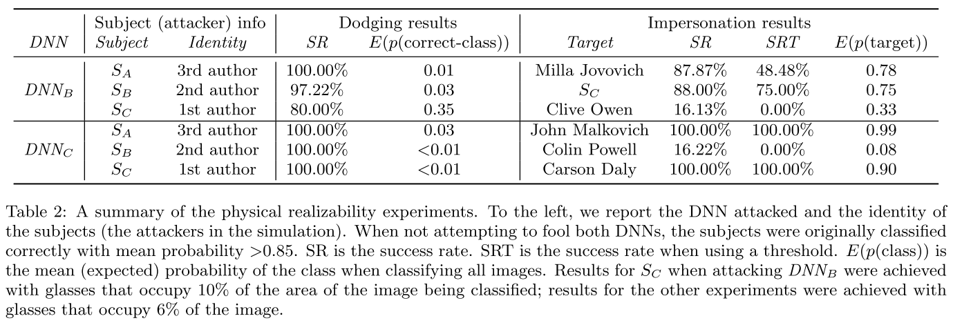
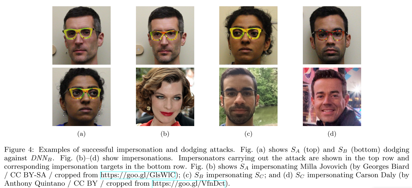
Against the Viola-Jones face detector
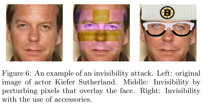
The original VJ detector utilizes a cascade of weak classifiers working on sub-windows of the whole image and rejects a sub-window in case one of its classifiers rejects it. A classifier in the cascade is formulated as:
Each weak classifier outputs either or based on the feature value and a threshold . The composed classifier decides whether it should be passed or not based on the threshold .
To make it differentiable, they utilize the sigmoid function and formulate the problem of generating adversarial perturbation for it as:
The VJ detector can be attacked, either, althought the perturbations are less inconspicuous than those in DNNA.
DAG - ICCV 2017
Cihang Xie1, Jianyu Wang, Zhishuai Zhang, Yuyin Zhou, Lingxi Xie, Alan Yuille. Adversarial Examples for Semantic Segmentation and Object Detection. ICCV 2017. arXiv:1703.08603
In this paper, we extend adversarial examples to semantic segmentation and object detection which are much more difficult.
It's a little different for generating adversarial examples against object detection system with region proposals, the latter works as a sampler and the perturbations are possibly destoried, leading to failures.
In experiments, we verify that when the proposals are dense enough on the original image, it is highly likely that incorrect recognition results are also produced on the new proposals generated on the perturbed image.
Problem formulation
This part is reorganized from the original paper
For the target system with classification score vector (before softmax normalization) as , the goal for object detection is to recognize a set of targets from an image with targets.
Each target is assigned to a ground-truth class label , the ground-truth for an image is .
To generate an adversarial example, the goal is to make the predictions of all targets go wrong with an additive adversarial perturbation :
To address this problem, an adversarial label is specified to each target. A random permutation function is designed to generate a set of adversarial labels .
The original loss function to minimize is written as:
The problem is then formulated as:
This problem is solved with a gradient descent algorithm proposed as DAG.
Dense Adversary Generation
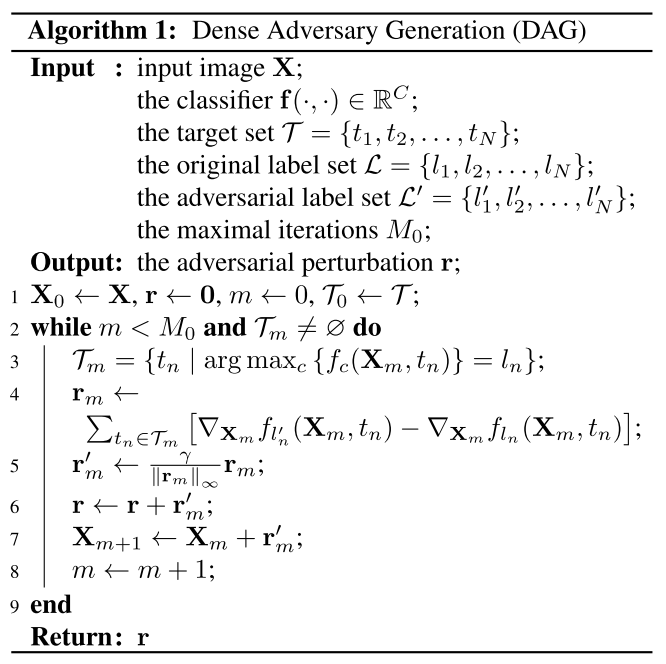
The strategy is explicit:
- Generate an adversarial label set according to the ground-truth label set .
- Find the set of correctly predicted targets for in -th iteration.
- Compute the gradient of loss respect to the input data for each target and accumulate these gradients as -th perturbation .
- Normalize the -th gradient.
- Accumulate -th perturbation to the final perturbation .
- Apply the -th perturbation to -th image to acquire .
- Iterate from 2 to 6
The threshold is loosen for dense proposals to generate a dense target set :
Technically, given the proposals generated by RPN, we preserve all positive proposals and discard the remaining. Here, a positive proposal satisfies the following two conditions: 1) the IOU with the closest ground-truth object is greater than 0.1, and 2) the confidence score for the corresponding ground-truth class is greater than 0.1.
Performance
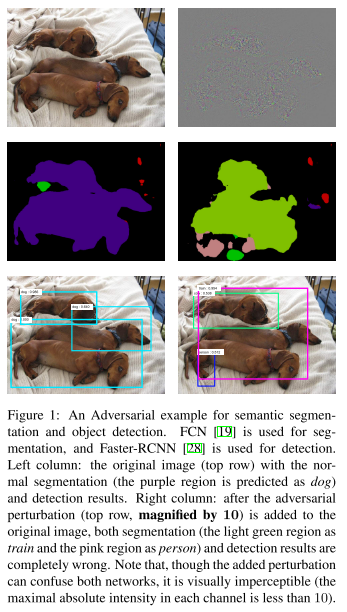
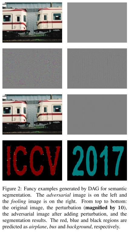
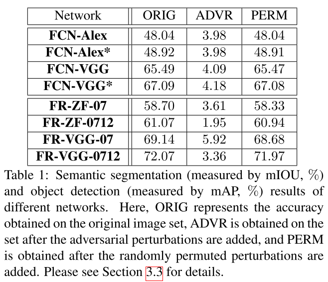
Transferability
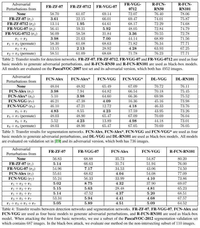
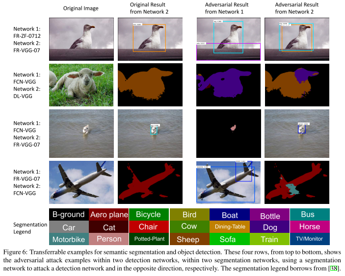
There are three transfering scenarios evaluated:
Cross-training
Apply the perturbations learned from one network to another network with the same architecture but trained on a different dataset.
Cross-network
Apply the perturbations learned from one network to another network with different architectures but trained on the same datatset.
Cross-task
Apply the perturbations generated by a detection network to a segmentation network or in the opposite direction.
Considering the cues obtained from previous experiments, we conclude that adversarial perturbations are closely related to the architecture of the network.
From the results listed in Tables 2– 4, we can observe that adding multiple adversarial perturbations often works better than adding a single source of perturbations.
Inspirations
This paper proves that the object detection and semantic segmentation system can be misled by adversarial examples, specificly interesting, we can mislead the semantic segmentation system to output a designated mask. They propose an iterative method called DAG, which ensembles adversarial perturbation for each target in image. The main techniques are the generation of false labels and densely cropping of proposals, the former provides the direction for optimization and the latter ensures the sampling of region proposal does not corrupt the adversarial pattern.
They also observe that the transferability of these adversarial examples is related to the network architecture and by ensembling the adversarial perturbations generated according to different network, the transferability is enhanced and the final perturbation is possible to attack a black-box model.
Based on the research, there are several possible future works to do:
- Steganography using adversarial examples - since we could use adversarial examples to control the shape of masks generated by semantic segmentation system, we could adapt it for steganography.
- Defend the attack of DAG - in most cases the exact of object is not required for object detection (e.g. it should be able to detect people in different clothes as "person"), so this kind of subtle noise is clearly removable while not hurting the mAP seriously.
- Realize the attack in physical world - all the attacks above are conducted in digital world, which make them not that practical, since the major scenario where object detection system and semantic segmentation system work is in physical world.
RP2 -CVPR 2018
Website: https://iotsecurity.eecs.umich.edu/#roadsigns
Kevin Eykholt, Ivan Evtimov, Earlence Fernandes, Bo Li, Amir Rahmati, Chaowei Xiao, Atul Prakash, Tadayoshi Kohno, Dawn Song. Robust Physical-World Attacks on Deep Learning Models. CVPR 2018 arXiv:1707.08945
Informed by the challenges above, we design Robust Physical Perturbations (RP2), which can generate perturbations robust to widely changing distances and angles of the viewing camera. RP2 creates a visible, but inconspicuous perturbation that only perturbs the object (e.g. a road sign) and not the object’s environment.
Problem formulation
Physical world presents several challenges compared to the digital world:
- Environmental conditions (perspectives vary from time to time)
- Spatial constraints (perturbations are unapplicable on background)
- Physical limits on imperceptibility (inconspicuous while catchable by cameras)
- Fabrication error (printing the generated perturbations introduces errors)
Taking account for these considerations, the final problem is formulated as:
The first part is a regularization term, in which is the generated perturbation and denotes a mask instantiating the spatial constraints. The NPS is the Non-Printability Score, in which is a set of printable colors and is a set of colors used in perturbation.
The last term is the normal goal for adversarial attack, where denotes the loss, is the original example, is the target label, denotes the mapping function that transforms the perturbation to the surface of object and is a set of examples under various transformations (mimicking environmental conditions).
Strategy
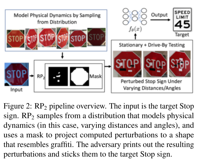
The concrete process is a little fuzzy in the paper:
- Generate a large distributions of stop signs to mimic the physical dynamics for further usage
- Select an input image from the distributions, merge it with masked and transformed version of current perturbation
- Feed the generated adversarial example into the classifier
- Optimize the perturbation according to the loss under regularization and printable constraints
Performance
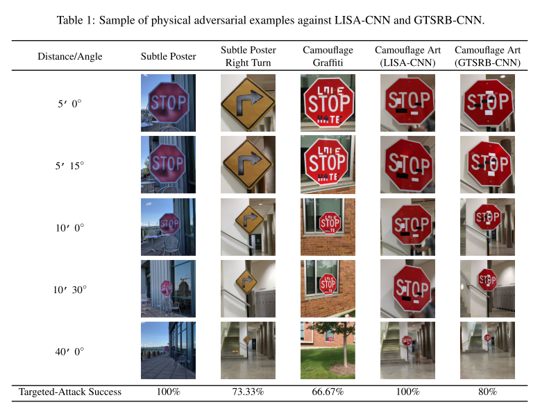
The LISA-CNN is trained over a U.S. traffic sign dataset (LISA) and the GTSRB-CNN is trained over the German Traffic Sign Recognition Benchmark (GTSRB).
LISA-CNN’s architecture is defined in the Cleverhans library and consists of three convolutional layers and an FC layer. It has an accuracy of 91% on the test set.
For GTSRB-CNN, they adopt the architecture of p2-TrafficSigns, and since they are in America:
Because we did not have access to German Stop signs for our physical experiments, we replaced the German Stop signs in the training, validation, and test sets of GTSRB with the U.S. Stop sign images in LISA. GTSRB-CNN achieves 95.7% accuracy on the test set. When evaluating GTSRB-CNN on our own 181 stop sign images, it achieves 99.4% accuracy.
Calculation of the attack success rate:
In which, is a set of clean images and is a set of perturbed images. The note denotes the image taken from distance and angle .
Inspirations
This was one of the pioneers to first apply adversarial example in physical world, thus the idea was inspiring. However, they targeted a classifier rather than a detector, which lowered the meaning of this problem and made the attack easier. The LISA sign dataset contains six thousands or so images of 47 classes and the GTSRB dataset contains 50000 images of 40 classes. The scale of these datasets is comparable to MNIST, which makes the classification of these data much more easier.
Adversarial patch - CVPR workshop 2019
Code: https://gitlab.com/EAVISE/adversarial-yolo
Thys S , Van Ranst W , Goedemé, Toon. Fooling automated surveillance cameras: adversarial patches to attack person detection. 2019 arXiv:1904.08653
The idea is to fool an object detection system (YOLOv2 in this paper) to overlook a human with adversarial patch.
Strategy
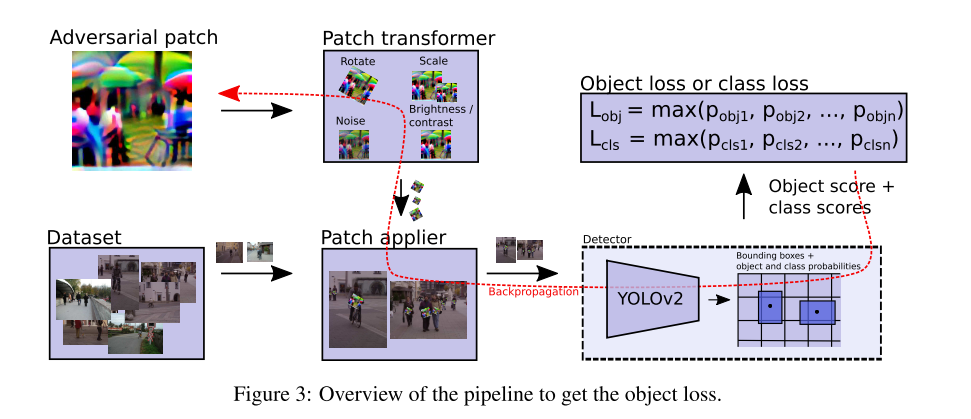
The strategy is quite explicit:
- Run the target person detector using normal images for bounding boxes
- Apply the current version of patch on a fixed relative position to bounding boxes with different transofrmations (to resist the variance of person gesture)
- Feed the resulting images and calculate the loss
- Changes pixels in the patch according to the loss (to maximize detection error)
Loss
The final loss function combines a non-printability loss, a total variation loss and an object loss.
The non-printability loss is designed to measure how well the colors can be represented by a common printer:
In which is a set of printable colors.
The total variation loss is designed to smooth the variance of color in patch:
The object loss is one of the losses in the detection system's training, but with a reversed optimization direction. It could be either a reversed classification loss, a reversed objectness loss or their combination.
Performance
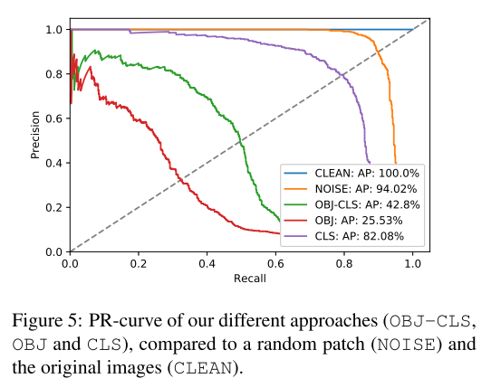
Inspirations
This idea is very interesting and points a potential direction for further possible attacks. Most traditional adversarial examples are constrained in the Lp norm sphere around normal examples, which make them very stealthier mathematically. While as this paper shows, a visible adversarial example is also very useful (or very dangerous in other words).
Adversarial T-Shirt - ECCV 2020
Kaidi Xu, Gaoyuan Zhang, Sijia Liu, Quanfu Fan, Mengshu Sun, Hongge Chen, Pin-Yu Chen, Yanzhi Wang, Xue Lin. Adversarial T-shirt! Evading Person Detectors in A Physical World. ECCV 2020. arXiv:1910.11099
The idea is to fool an object detection system (YOLOv2 and Faster R-CNN in this paper) to overlook a human with a T-shirt, on which there are adversarial patches.
Problem definition
From the recorded video (i.e. where a man walking casually with checkboard), video frames, , are extracted. The adversarial T-shirt is characterized by , where is a bounding box of the cloth region for perturbations in th frame, denotes the element-wise product, and is the universarial perturbation applide to .
The goal of adversarial T-shirt is to design such that the perturbed frames of are mis-detected by object detectors.
Strategy
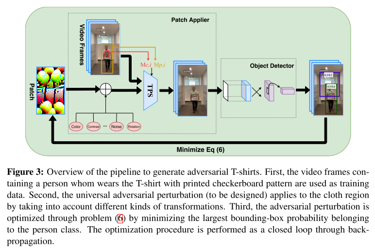
The strategy is explicit:
- Record a video of a man wearing a T-shirt with a checkboard image (printed on the area where adversarial patch is to be applied) walking casually
- Map the current adversarial patch into the T-shirt in video using TPS, considering multiple transformations
- Feed the generated video to the detector for calculation of loss
- Optimize the adversarial patch according to the loss
Patch applier
Considering physical transformations, the th perturbed frame is calculated as:
In which, is the bounding box for person and is the bounding box for cloth region.
Taking the following three physical transformations into account:
- TPS transformation (applied to adversarial patch )
- physical color transformation (converts digital color into printable color)
- convetional physical transformation (applied to the region within the bounding box for person)
Here denotes the set of possible non-rigid transformations, is given by a regression model learnt from the color spectrum in the digital space to its printed counterpart, and denotes the set of commonly-used physical transformations, e.g., scaling, translation, rotation, brightness, blurring and contrast.
The final equation to calculate is as follows:
is an additive Gaussian noise that allows the variation of pixel values, where is a given smoothing parameter and we set it as 0.03 in our experiments such that the noise realization falls into the range [−0.1, 0.1].
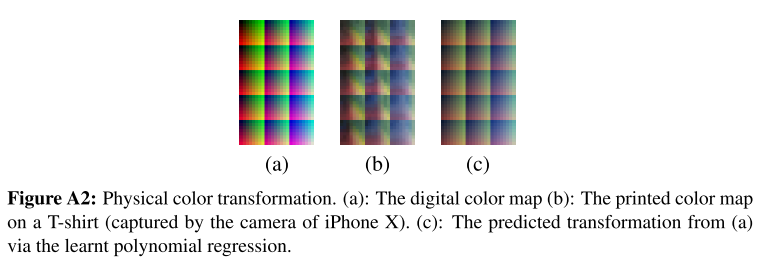
We learn the weights of the quadratic polynomial regression by minimizing the mean squared error of the predicted physical color (with the digital color in Figure A2 (a) as input) and the ground-truth physical color provided in Figure A2(b).
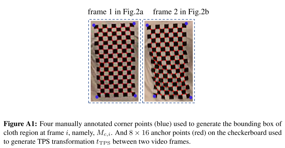
We first manually annotate four corner points (see blue markers in Figure A1) to conduct a perspective transformation between two frames at different time instants. This perspective transformation is used to align the coordinate system of anchor points used for TPS transformation between two frames.
Thin Plate Spline mapping
Previous methods have considered multiple transformations of the adversarial examples before fed to the target system, including perspective transformation, brightness adjustment, resampling, smoothing and saturation. However, cloth deformation due to movements of human body is a little different, since TPS is used to model this transformation.
Given a set of control points with locations on image , TPS provides a parametric model of pixel displacement when mapping to :
In which, and are the TPS parameters, represents the displacement along either or direction.
Given the locations of control points on the transformed image , , TPS resorts to a regression problem to determine the parameters. The regression problem can be solved by the following linear system of equations:
In which, , , and , .
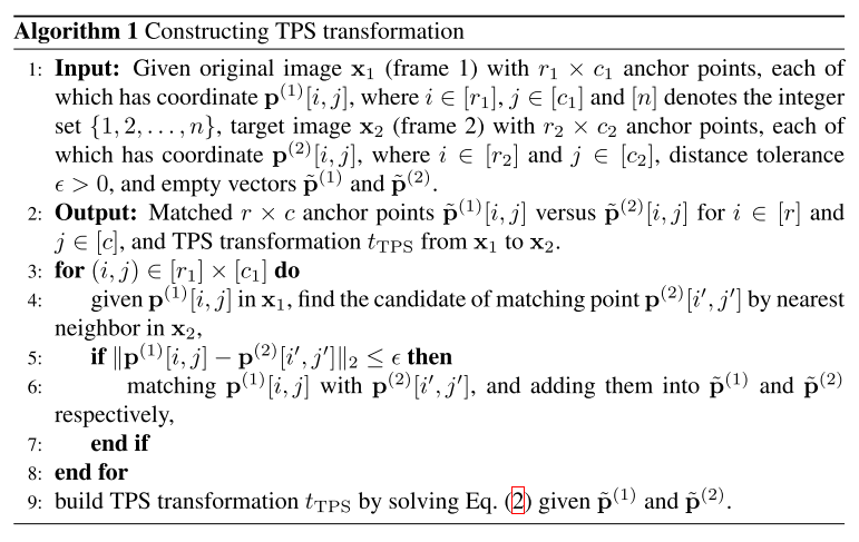
The construction of two set of control points is conducted as Algorithm 1.
I do not really understand how it works yet. From my current understanding, this is a sophisticated linear map, not very different from a single layer of nueral networks.
Problem formulation
The EoT formulation to fool a single object detector is cast as:
In which, is an attack loss for misdetection and is the total-variation norm enhancing perturbations' smoothness.
In the formulation of , is the confidence score for th bounding box, is a confidence threshold, is the th bounding box, is the known bounding box for person. The indicator filters out predicted bounding boxes with intersection of the bounding box of person in th frame higher than .
For fooling mutiple object detectors, a physical ensemble attack is utilized. Given object detectors associated with attack loss functions , the problem is formulated as:
In which, are domain weights adjusting the importance of each object detector and is a probabilistic simplex (i.e. ).
Performance
These are evaluations under the metric of Attack Success Rate.
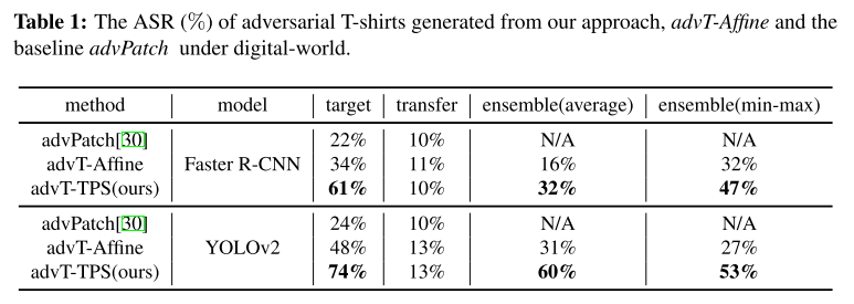
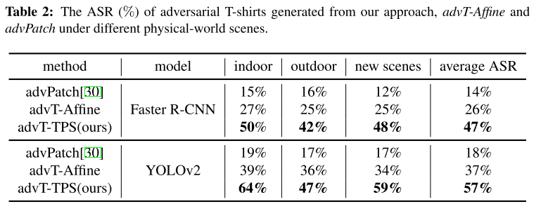
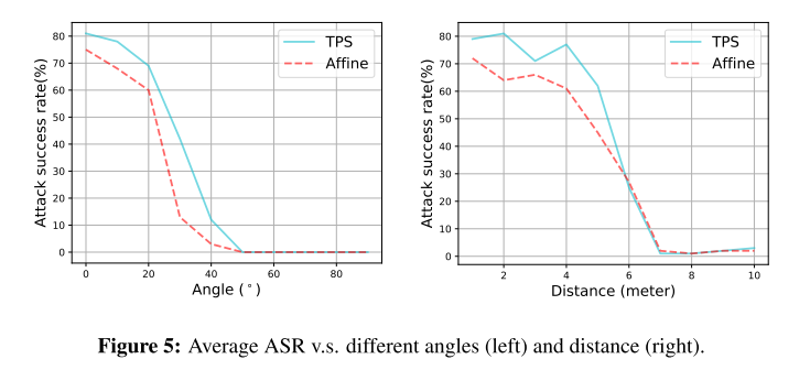

The baseline denoted as advPatch is the method proposed in Fooling automated surveillance cameras: adversarial patches to attack person detection. The other method called advT-Affine is the same method with TPS process replaced by affinement.
Inspirations
It's really a great idea to use a T-shirt to carry the adversarial patterns. This paper walks through a whole process of defining problem, formulating problem and solving problem, which also leaves a large space for future research.
Given the reported performance, there are several possible improvements following this trajectory:
- Increase the attack success rate (the current ASR is relatively low)
- Cope with the problem of different angles and different scales (the reported ASR is low in different angles and small resolutions)
- Better algorithms to replace TPS (TPS is a very tarditional method)
- Defend the attack of adversarial T-shirts (which is not that meaningful yet, since the T-shirt itself is relatively weak)
If ASR is increased tremendously and the problem of angle and scale is solved, the generated T-shirt will be a very good merchandise.
Invisibility cloak - ECCV 2020
Zuxuan Wu, Ser-Nam Lim, Larry Davis, Tom Goldstein. Making an Invisibility Cloak: Real World Adversarial Attacks on Object Detectors. ECCV 2020. arXiv:1910.14667
The idea of this paper is basically the same as that in adversarial T-shirt, but the approach is a little different, and it seems to have better results.
Defense
Towards Adversarially Robust Object Detection - ICCV 2019
Paper: ICCV 2019- Towards Adversarially Robust Object Detection
Haichao Zhang, Jianyu Wang. Towards Adversarially Robust Object Detection. Proceedings of the IEEE/CVF International Conference on Computer Vision (ICCV), 2019, pp. 421-430
We show that it is possible to improve the robustness of the object detector w.r.t.various types of attacks and propose a practical approach for achieving this, by generalizing the adversarial training framework from classification to detection.
One-stage object detector
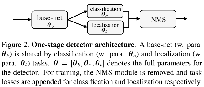
An object detector takes an image as input and outputs a varying number of detected objects, each represented by a probability vector over classes and a bounding box . Non-maximum suppression (NMS) is a prevailing post-process to remove redundant detections.
The general structure of an one-stage detector is shown as Figure 2. The training of a detector parameterized by is formulated as:
Which is to minimize the expectation of loss over a given labeled training images . But in practice (c.f. Figure 2), the problem is reformed as a combination of classification and regression:
The different parts of the output from are used for classification and regression of locations, which is essentially an instance of multi-task learning.
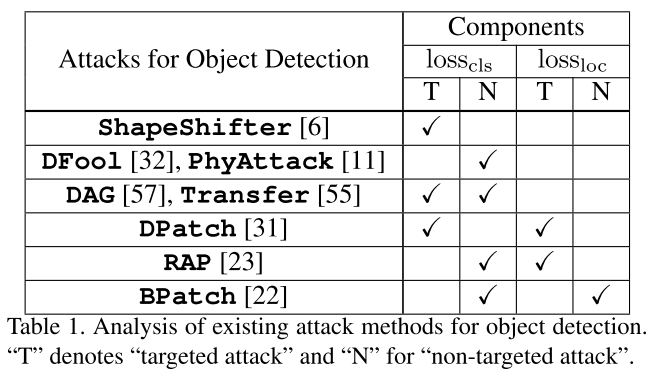
All of the proposed attacks against object detector are either targeted to undividual task losses or their combination. The effectiveness of attacking by individual loss can be explained by the shared base net of these two branches and the shared post-process (i.e. NMS) merging two branches.
Observation
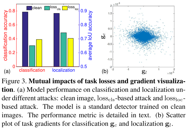
For classification, we compute the classification accuracy on the candidate set.
For localization, we compute the average IoU of the predicted bounding boxes with groundtruth bounding boxes.
The attack is generated with onestep PGD and a budget of 8
Our first empirical observation is that different tasks have mutual impacts and the adversarial attacks trailered for one task can reduce the performance of the model on the other task
Our second empirical observation is that the gradients of the two tasks share certain level of common directions but are not fully aligned, leading to misaligned task gradients that can obfuscate the subsequent adversarial training
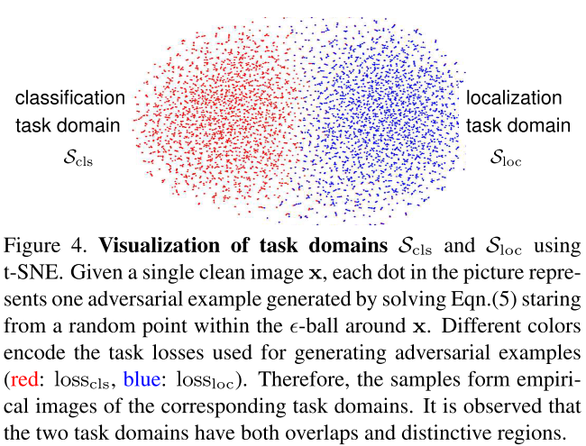
They discover that these two losses are correlated, i.e. attacking one loss affects another loss. But the magnitudes of the gradients of these losses are different (misaligned, c.f. Figure 3(b)), and the adversarial examples generated targeted to these losses are also partially overlapped.
Adversarial training for robust detection
Based on the observation, they proposed the following adversarial training for object detection:
In which, and is the task-oriented domain:
In which, and , which is the -ball centered around the clean image with a radius of perturbation budget .
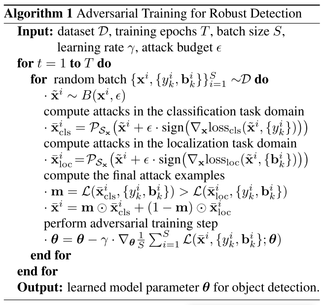
This problem is solved using PGD (Projected Gradient Descent) as shown in Algorithm 1, the denotes projecting back into the feasible region .
In short, the strategy is to separately attack classification loss and localization loss and train the model over the best adversarial example considering both two branches based on the adversarial examples obtained separately.
But the algorithm does not persue for the optimal solution, the inner problem is solved using projected FGSM.
Performance
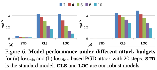
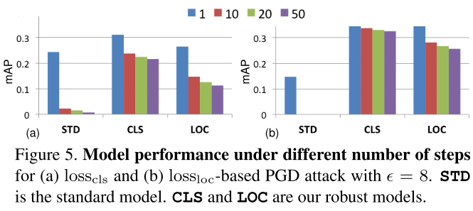
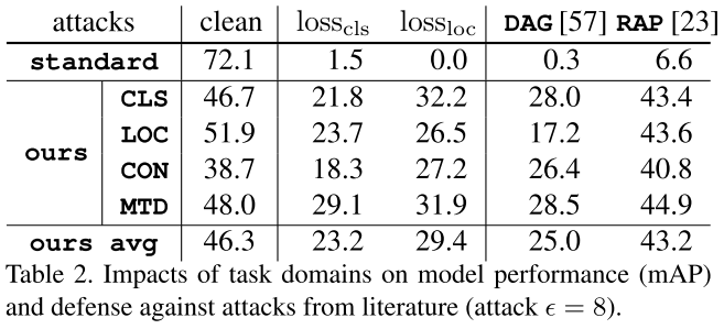

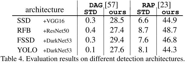
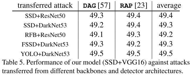
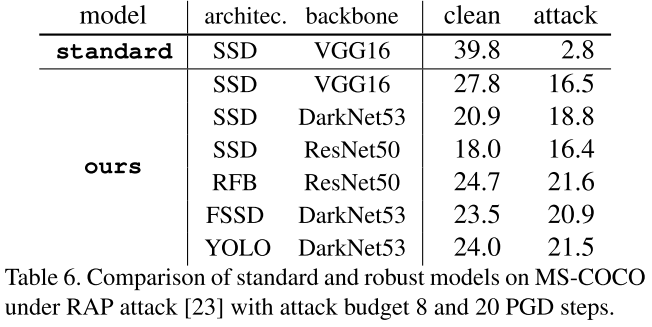
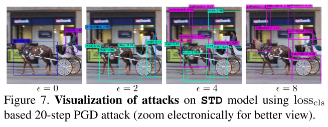
They use SSD in general experiments before cross backbone evaluation. They use PASCAL VOC 07+12 trainval and MS-COCO 2014 trainval as the dataset for experiments. All models are trained from scratch and for adversarial training, the budget is set to 8.
The notations are as follows:
- STD: standard training with clean image as the domain
- CLS: using only as the task domain for training
- LOC: using only as the task domain for training
- CON: using the conventional task agnostic domain
- MTD: using the task oriented domain