Adversarial Defense at Inference

By LI Haoyang 2020.11.12

Content

Purification

PixelDefend - ICLR 2018

This defense is breached in Obfuscated Gradients Give a False Sense of Security - ICML 2018.

Yang Song, Taesup Kim, Sebastian Nowozin, Stefano Ermon, Nate Kushman. PixelDefend: Leveraging Generative Models to Understand and Defend against Adversarial Examples. ICLR 2018. arXiv:1710.10766

In this paper, we show empirically that adversarial examples mainly lie in the low probability regions of the training distribution, regardless of attack types and targeted models.

They argue that adversarial examples lie in the low probability region of the generating distribution of datasets, therefore they fool the classifiers mainly due to covariate shift.

This is analogous to training models on MNIST (LeCun et al., 1998) but testing them on Street View House Numbers (Netzer et al., 2011).

Pixel CNN

The PixelCNN (van den Oord et al., 2016b; Salimans et al., 2017) is a generative model with tractable likelihood especially designed for images.

It defines the joint distribution over all pixels by factorizing it into a product of conditional distributions, i.e.

p_{CNN}(\bold{X})=\prod_{i}p_{CNN}(x_i|x_{1:(i-1)})

The pixel dependencies are in raster scan order (i.e. row by row and column by column with each row).

It views an image as a vector of pixels and predicts the next pixel with the previous pixel sequentially.

$I\times J$ $K$ channels, its bits per dimension is defined as

BPD(\bold{X})\stackrel{\Delta}{=}-\text{log}p_{CNN}(\bold{X})/(I\times J\times K\times log2)

Distribution of adversarial examples

The transferability of adversarial examples indicate that there are some intrinsic properties of adversarial examples which are classfier-agnostic.

One possibility is that, compared to normal training and test images, adversarial examples have much lower probability densities under the image distribution.

As a result, classifiers do not have enough training instances to get familiarized with this part of the input space.

They train a PixelCNN on CIFAR-10 and use its log-likelihood as an approximation to the true underlying probability density. They also generate a bunch of adversarial examples respect to ResNet.

As shown in Figure 2, the distribution of log-likelihoods show considerable difference between perturbed images and clean images. As for the random noise that also shift the distribution of original data (but not adversarial), they explain that

We believe this is due to an inductive bias that is shared by many neural network models but not inherent to all models, as discussed further in Appendix A

$p$ -value is a statistical indicator calculated from PixelCNN model, for clean images, it should follow a uniform distribution. As shown in Figure 3, there are clear differences between the uniform distribution and the distributions of adversarial examples.

Purifying images with PixelDefend

The purification is intended to move the adversarial examples back towards the training distribution.

$\bold{X}^*$ $p(\bold{X})$ $\bold{X}^*$ $\epsilon_{defend}$ $\bold{X}$ , i.e.

\max_{\bold{X^*}}p(\bold{X}^*)\\ s.t.\ ||\bold{X}^*-\bold{X}||_{\infty}<\epsilon_{defend}

$\epsilon_{defend}$ $p(\bold{X})$ $p_{CNN}(\bold{X})$ from the trained PixelCNN.

They test L-BFGS-B and a greedy technique (as in Algorithm 1) to solve this problem.

As shown above, PixelDefend can effectively purify the adversarial examples.

$\epsilon_{defend}$ to deal with this problem.

They argue that the ability to attack end-to-end with PixelDefend is limited (although disputable).

Experiments

Inspirations

The idea of purifying adversarial example is very ideal and if it was not breached and classified as gradient masking.

I think this road is still possible, perhaps combining adversarial training with purification of adversarial examples.

Mixup Inference

Post-averaging - 2019

Yuping Lin, Kasra Ahmadi K. A., Hui Jiang. Neural Networks Against Adversarial Attacks. arXiv preprint 2019. arXiv:1905.12797

This paper is likely to have been rejected by NIPS 2019.

We first explicitly compute the Fourier transform of deep ReLU neural networks and show that there exist decaying but nonzero high frequency components in the Fourier spectrum of neural networks.

We demonstrate that the vulnerability of neural networks towards adversarial samples can be attributed to these insignificant but non-zero high frequency components.

We propose to use a simple post-averaging technique to smooth out these high frequency components to improve the robustness of neural networks against adversarial attacks.

Fourier Analysis of Neural Networks

As we know, any fully-connected ReLU neural networks (prior to the softmax layer) essentially form piece-wise linear functions in input space.

Definition 2.1. $f:\R^n\to\R$ $\R^n$ $M$ $\mathfrak{R}_m$ $m=1,2,\dots,M$ $f$ is linear:

f(\bold{x})=\begin{cases} \bold{w}_1\cdot\bold{x}&\bold{x}\in\mathfrak{R}_1\\ \bold{w}_2\cdot\bold{x}&\bold{x}\in\mathfrak{R}_2\\ \cdots\\ \bold{w}_M\cdot\bold{x}&\bold{x}\in\mathfrak{R}_M\\ \end{cases}

Lemma 2.2. Composition of a piece-wise linear function with a ReLU activation function is also a piece-wise linear function.

Theorem 2.3. The output of any hidden unit in an unbiased fully-connected ReLU neural network is a piece-wise linear function.

It states that if we take out the neural networks with ReLU activation cut in the chosen unit, the function it forms is a piece-wise linear function.

For the purpose of mathematical analysis, we need to decompose each region into a union of some well-defined shapes having a uniform form, which is called infinite simplex.

Definition 2.4. $\bold{V}=\{\bold{v}_1,\bold{v}_2,\dots,\bold{v}_n\}$ $n$ $\R^n$ $\mathfrak{R}_{\bold{V}}^{+}$ $\bold{V}$ using only positive weights:

\mathfrak{R}_{\bold{V}}^{+}=\left\{\sum_{k=1}^n\alpha_k\bold{v}_k|\alpha_k>0,k=1,2,\dots,n\right\}

$\{(0,1),(1,0)\}$ .

$\bold{V}$ can be interpreted as a set of bases.

Theorem 2.5. $f(\bold{x})$ $f(\bold{x})=\sum_{l=1}^L f_l(\bold{x})$ , each of which is linear and non-zero only in an infinite simplex as follows:

f_l(\bold{x})=\begin{cases} \bold{w}_l\cdot\bold{x}&\bold{x}\in\mathfrak{R}_{\bold{V}_l}^{+}\\ 0&otherwise \end{cases}

$\bold{V}_l$ $n$ $\bold{w}_l$ is a weight vector.

$\bold{x}$ $U_n=[0,1]^n$ .

$f_l(\bold{x})$ $\prod_{r=1}^n h(x_r)h(1-x_r)$ $h(x)$ is the Heaviside step function (阶跃函数).

I think this is a clamp, not a normalization....

$n^2$ $\bold{x}$ $\mathfrak{R}_{\bold{V}_q}^{+}$ .

$\mathfrak{R}_{\bold{V}_q}^{+}$ $\bold{x}$ $r_q$ .

$x_{r_q}$ $\mathfrak{R}_{\bold{V}_q}^{+}$ .

Why?

$f(\bold{x})=\sum_{q=1}^Qg_q(\bold{x})$ $g_q(\bold{x})(q=1,2,\dots,Q)$ has the following form:

g_q(\bold{x})=\begin{cases} \bold{w}_q\cdot\bold{x} h(1-x_{r_q})&\bold{x}\in\mathfrak{R}_{\bold{V}_q}^{+}\\ 0&otherwise \end{cases}

$\bold{V}_q$ $g_q(\bold{x})$ $\bold{V}_{*}=\{\bold{e}_1,\cdots,\bold{e}_n\}$ as follows:

g_q(\bold{x})=\begin{cases} \overline{\bold{w}}_q\cdot\overline{\bold{x}}_q h(1-\bold{1}\cdot \overline{\bold{x}}_q)&\overline{\bold{x}}_q\in\mathfrak{R}_{\bold{V}_{*}}^{+}\\ 0&otherwise \end{cases}

$\overline{\bold{x}}_q=\bold{x}\bold{A}_q^\top$ $\overline{\bold{w}}_q=\bold{w}_q\bold{A}_{q}^{-1}$ .

Lemma 2.6. Fourier transform of the following function:

s(\bold{x})=\begin{cases} h(1-\bold{1}\cdot\bold{x})&\bold{x}\in\mathfrak{R}_{\bold{V}_*}^{+}\\ 0&otherwise \end{cases}

may be represented as:

S(w)=(\frac{-i}{\sqrt{2\pi}})^n\sum_{r=0}^n\frac{e^{-iw_r}}{\prod_{r^\prime\neq r}(w_{r^\prime}-w_r)}

$w_r$ $r$ $w(r=1,\dots,n)$ $w_0=0$ .

Finally we derive the Fourier transform of fully-connected ReLU neural networks as follows.

Theorem 2.7. $\sum_{q=1}^Q\bold{w}_q\bold{A}_q^{-1}\nabla S(w\bold{A}_q^{-1})$ $\nabla$ denotes the differential operator.

Obviously, neural networks are the so-called approximated bandlimited models as defined in (Jiang, 2019), which have decaying high frequency components in Fourier spectrum.

$\bold{A}_q$ $\mathfrak{R}_{\bold{V}_q}^{+}$ $\R^n$ $\mathfrak{R}_{\bold{V}_q}^{+}$ $\bold{A}_q^{-1}$ have a large determinant and contribute to the high frequency components a lot.

Understanding Adversarial Examples

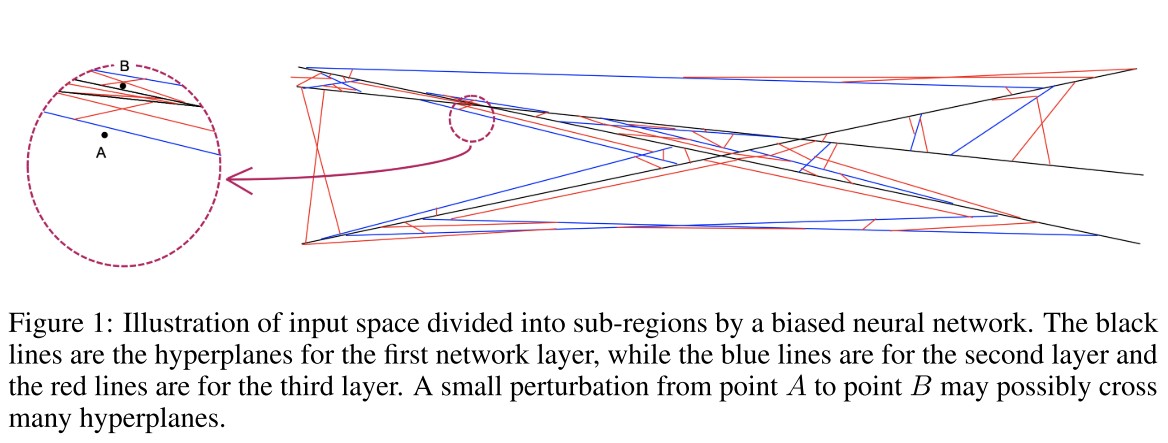
According to Theorem 2.3., a neural network may be viewed as a sequential devision of the input space as shown in Figure 1. Each layer is a further division of the existing regions from the previous layers.

Hence a neural network with multiple layers would result in a tremendous amount of sub-regions in the input space.

When we learn a neural network, we can not expect there is at least one sample inside each region. For those regions that do not have any training sample, the resultant linear functions in them may be arbitrary since they do not contribute to the training objective function at all.

When we measure the expected loss function over the entire space, their contributions are negligible since the chance for a randomly sampled point to fall into these tiny regions is extremely small.

Given that the total number of regions is huge, those tiny regions are almost everywhere in the input space.

They attribute adversarial examples to the existence of these untrained arbitrary small regions almost everywhere.

$\Delta x$ $\bold{x}$ , the fluctuation in the output of any hidden node can be approximately represented as:

\Delta f(\bold{x})\propto N\cdot\prod_{l}\bold{E}\left[|\bold{v}_{ij}^{(l)}|\right]

$N$ $\bold{x}$ $\bold{x}+\Delta\bold{x}$ .

$\bold{x}$ in a high-dimensional space, we can always move it to cross a large number of hyperplanes to enter a tiny region.

$N$ is fairly large, the above equation indicates that the output of a neural network can still fluctuate dramatically even after all weight vectors are regularized by L1 or L2 norm.

In principle, neural networks must be strictly bandlimited to filter out those decaying high frequency components in order to completely eliminate all adversarial samples.

Post-averaging

The post-averaging proposed works by averaging the output of a series of data points. It is computed as an integral over a small neighborhood centered at the input:

f_C(\bold{x})=\frac{1}{\bold{V}_C}\int\cdots\int_{\bold{x}^\prime\in C}f(\bold{x}-\bold{x}^\prime)d\bold{x}^\prime

$\bold{x}$ $f(\bold{x})$ $C$ $\bold{V}_C$ denotes its volume.

It seems that if the error rate of this model in this neighborhood is smaller than 0.5, this will works fine.

$C$ $n$ $\R^n$ $r$ $f_C(\bold{x})$ is:

F_C(w)=F(w)\frac{1}{\bold{V}_C}\int\cdots\int_{\bold{x}^\prime\in C}e^{-i\bold{x}^\prime\cdot w}d\bold{x}^\prime=F(w)=\frac{\Gamma(\frac{n}{2}+1)}{\pi^{\frac{n}{2}}}\frac{J_{\frac{n}{2}}(r|w|)}{(r|w|)^{\frac{n}{2}}}

$J_{\frac{n}{2}}(\cdot)$ $n/2$ .

$J_v(w)$ $1/\sqrt{w}$ $|w|\to\infty$ $F_C(w)\sim\frac{F(w)}{(r|w|)^{\frac{n+1}{2}}}$ $|w|\to\infty$ .

$r$ is chosen properly, the post-averaging operation can significantly bandlimit neural networks by smoothing out high frequency components.

Sampling Methods

The integral is intractable in practice. They propose an approximation.

$\bold{x}$ $K$ $C$ $\bold{x}$ $\{\bold{x}_1,\bold{x}_2,\cdots,\bold{x}_K\}$ , the integral is approximated with

f_C(\bold{x})\approx\frac{1}{K}\sum_{k=1}^{K}f(\bold{x}_k)

$\hat{\bold{v}}$ , the samples are taken by

\bold{x}^\prime=\bold{x}+\lambda\cdot\hat{\bold{v}}

$\lambda=[\pm\frac{r}{3},\pm\frac{2r}{3},\pm r]$ $\hat{\bold{v}}$ is a selected unit-length directional vector.

They propose two sampling strategies:

random
Fill the directional vectors with random noise.
A post Gaussian noise augmentation.
approx
Approximate the directional vectors with gradient.
A post DeepFool augmentation.

Experiments

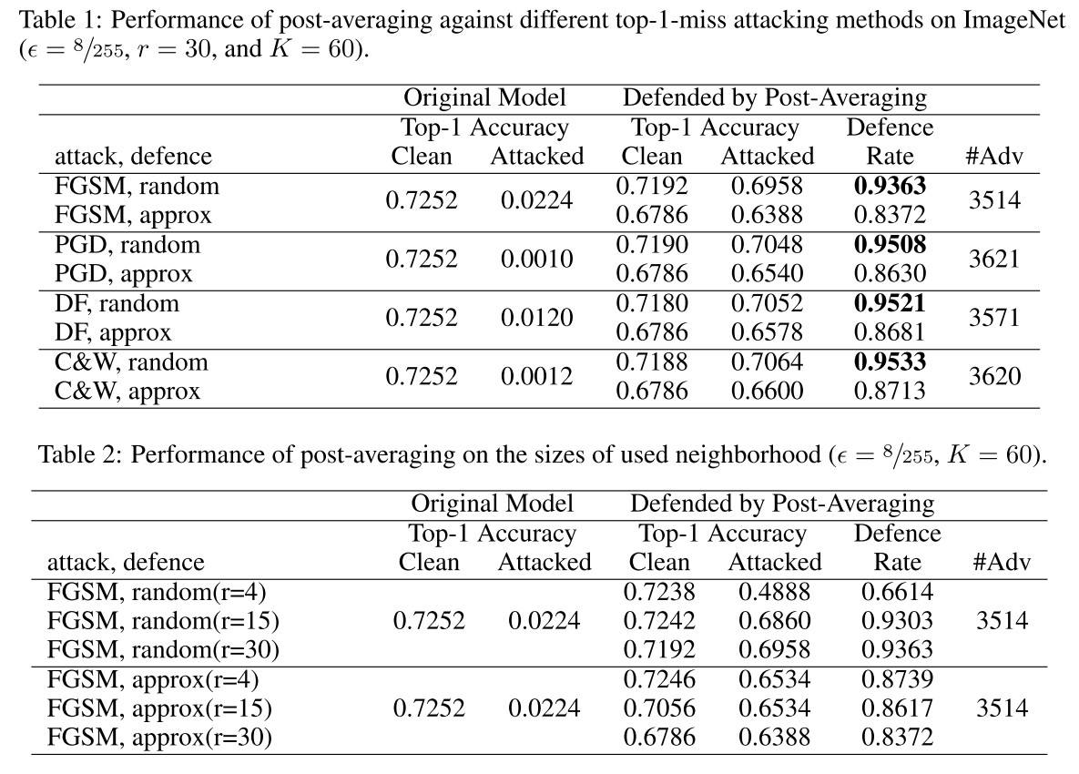
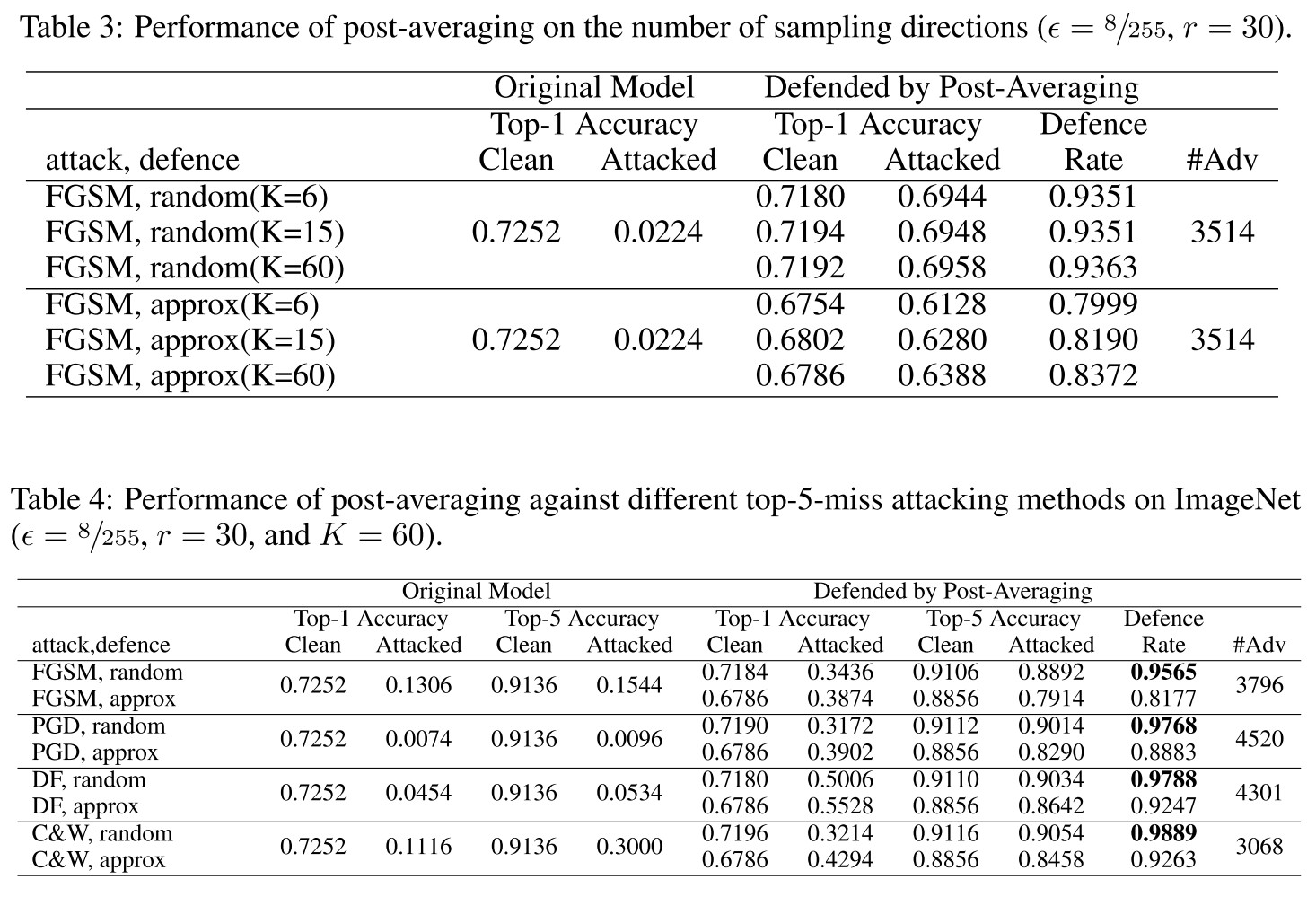
The proposed method requires no re-training, so they used a pre-trained VGG16 network. For evaluation, they adopt Foolbox to generate adversarial examples.

$\ell_{\infty}$ $\epsilon=8/255$ .

The results are too good to be true....

Inspirations

Their explanation for adversarial examples are unique and inspiring, the defense is reported to be very effective.

The post-averaging seems to be time-consuming, which hinders its application.

Mixup Inference - ICLR 2020

Code: https://github.com/P2333/Mixup-Inference

Paper: https://openreview.net/forum?id=ByxtC2VtPB

Tianyu Pang, Kun Xu, Jun Zhu. Mixup Inference: Better Exploiting Mixup to Defend Adversarial Attacks. ICLR 2020.

Namely, since the locality of the adversarial perturbations, it would be more efficient to actively break the locality via the globality of the model predictions.

MI mixups the input with other random clean samples, which can shrink and transfer the equivalent perturbation if the input is adversarial.

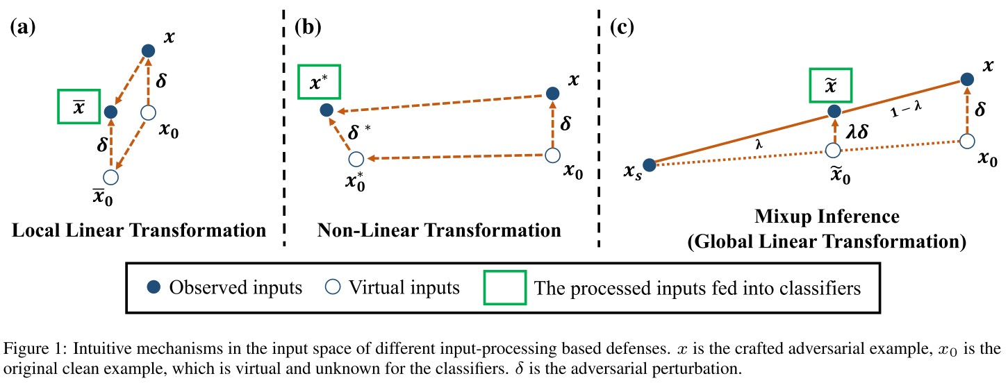
As shown in Figure 1(c), mixup inference introduces pertubation shrinkage and input transfer to the potentially perturbed examples.

$x$ $x_s$ $\tilde{x}=\lambda x+(1-\lambda)x_s$ .

Mixup Inference defense

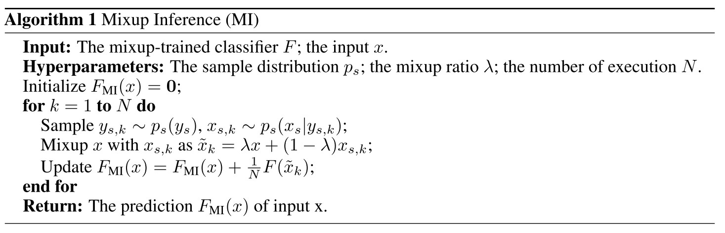
An iteration of MI operations is as follows:

$y_s\sim p_s(y)$ .
$x_s$ $p_s(x|y_s)$ .
$x$ $\tilde{x}=\lambda x+(1-\lambda)x_s$ .
$F_{MI}(x)$ .

They actually construct a new statistical model based on the original model.

Theoretical analysis

$z$ defined as

z=\begin{cases} 1,&\text{ if }x\text{ is adversarial}\\ 0,&\text{ if }x\text{ is clean} \end{cases}

$x_0$ $p(x)$ . A general example can be denoted as

x=x_0+\delta\cdot \bold{1}_{z=1}

$x_0+\delta\notin \text{supp}(p(x))$ .

$H(x_i)$ $y_i$ $H_y(x_i)=\bold{1}_{y=y_i}$ .

$x_0+\delta$ $G(\delta;x_0)$ $F$ $x$ is off the data manifolds.

$x$ , the prediction vector is

F(x)=F(x_0+\delta\cdot\bold{1}_{z=1})=H(x_0)+G(\delta;x_0)\cdot\bold{1}_{z=1}

$\tilde{x}$ in MI is then

\begin{array}{rl} F(\tilde{x})&=H(\tilde{x}_0)+G(\lambda\delta;\tilde{x}_0)\cdot\bold{1}_{z=1}\\ &=\lambda H(x_0)+(1-\lambda)H(x_s)+G(\lambda \delta;\tilde{x}_0)\cdot\bold{1}_{z=1} \end{array}

$H$ is a linear function on the combination of clean images.

$F_{MI}(x)$ $\Bbb{E}_{p_s}[F(\tilde{x})]$ , i.e.

F_{MI}(x)=\frac{1}{N}\sum_{i=1}^N F(\tilde{x}_i)\stackrel{\infty}{\to}\Bbb{E}_{p_s}[F(\tilde{x})]

$\forall k\in[L]\backslash \{y\}$ .

\Bbb{E}_{y_s\sim\mathcal{U}_{\hat{y}}(y)}\Bbb{E}_{x_s\sim p_s(x|y_s)}[F_y-F_k]>0\implies \lambda> L^{-1}

$y$ $F(\cdot)$ are

\begin{array}{rl} F_y(x)&=1+G_y(\delta;x_0)\cdot\bold{1}_{z=1}\\ F_y(\tilde{x})&=\lambda+(1-\lambda)\cdot\bold{1}_{y=y_s}+G_y(\lambda\delta;x_0)\cdot\bold{1}_{z=1} \end{array}

$\hat{y}=F(x)$ $\hat{y}$ $F(\cdot)$ are

\begin{array}{rl} F_{\hat{y}}(x)&=\bold{1}_{z=0}+G_{\hat{y}}(\delta;x_0)\cdot\bold{1}_{z=1}\\ F_{\hat{y}}(\tilde{x})&=\lambda\cdot\bold{1}_{z=0}+(1-\lambda)\cdot\bold{1}_{\hat{y}=y_s}+G_{\hat{y}}(\lambda\delta;\tilde{x}_0)\cdot\bold{1}_{z=1} \end{array}

$\bold{1}_{y=\hat{y}}=\bold{1}_{z=0}$ .

Consider the following scenarios:

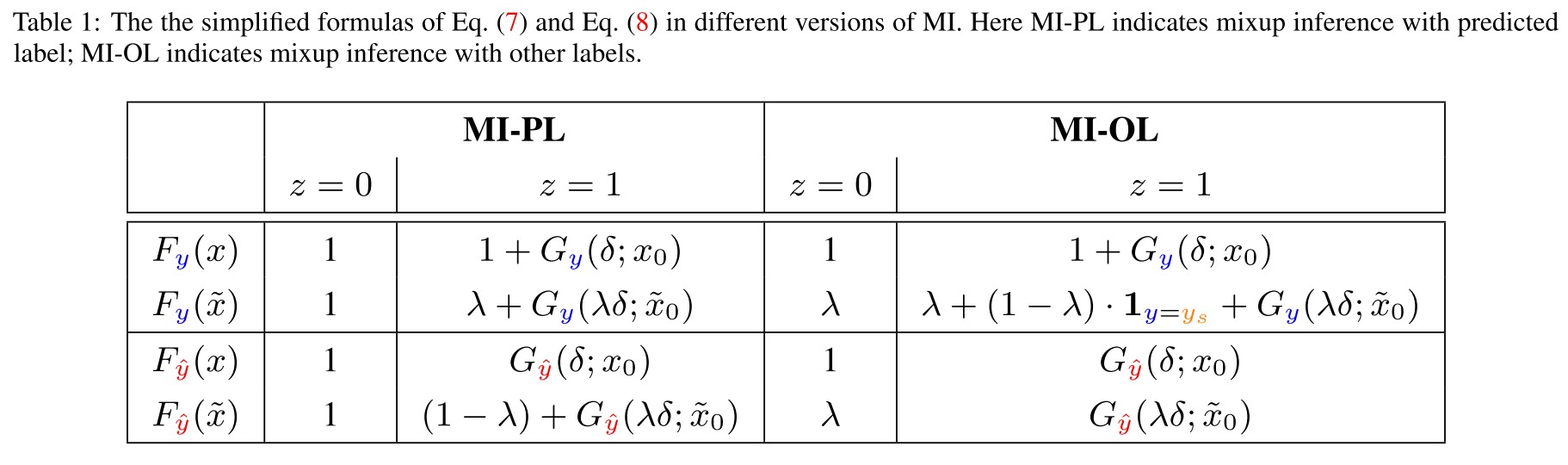
MI with predicted label (MI-PL)
$y_s$ $\hat{y}$ $p_s(y)=\bold{1}_{y=y_s}$ .
MI with other labels (MI-OL)
$y_s$ $\tilde{y}$ $p_s(y)=\mathcal{U}_{\tilde{y}}(y)$ $\{y\in[L]|y\neq \hat{y}\}$ .

The resulting output is shown below.

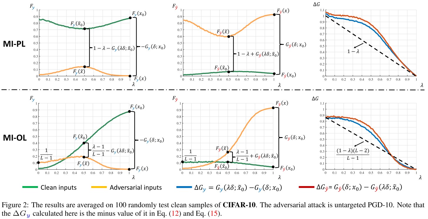
Consider the difference:

\Delta F(x;p_s)=F_{MI}(x)-F(x)\stackrel{\infty}{\to}\Bbb{E}_{p_s}[F(\tilde{x})]-F(x)

$y$ $\hat{y}$ $z=1$ ).

Named as robustness improving condition (RIC) and formally denoted as

\Delta F_y(x;p_s)|_{z=1}>0;\Delta F_{\hat{y}}(x;p_s)|_{z=1}<0

They also define a detection gap (DG), denoted as

\Bbb{DG}=\Delta F_{\hat{y}}(x;p_s)|_{z=1}-\Delta F_{\hat{y}}(x;p_s)|_{z=0}

$\Delta F_{\hat{y}}(x;p_s)$ is better as a detection metric.

MI with predicted label (MI-PL)

If MI-PL can improve the general-purpose robustness, it should satisfy RIC, according to Table 1, it means that

\Bbb{E}_{x_s\sim p_s(x|\hat{y})}[G_k(\delta;x_0)-G_k(\lambda\delta;\tilde{x}_0)]=\begin{cases} >1-\lambda,&\text{ if }k=\hat{y}\\ <\lambda- 1, &\text{ if }k=y \end{cases}

The upper notion can be decomposed into

\underbrace{\Bbb{E}_{x_s\sim p_s(x|\hat{y})}[G_k(\delta;x_0)-G_k(\delta;\tilde{x}_0)]}_{\text{input transfer}}+\underbrace{\Bbb{E}_{x_s\sim p_s(x|\hat{y})}[G_k(\delta;\tilde{x_0})-G_k(\lambda\delta;\tilde{x}_0)]}_{\text{perturbation shrinkage}}

Indicating the two mechanisms of MI.

And the detection gap is

\Bbb{DG}_{MI-PL}=\Bbb{E}_{x_s\sim p_s(x|\hat{y})}[G_{\hat{y}}(\delta;x_0)-G_{\hat{y}}(\lambda\delta;\tilde{x}_0)]-(1-\lambda)

MI with other labels (MI-OL)

$\Bbb{E}(\bold{1}_{y=y_s})=\frac{1}{L-1}$ , similarly, there should exist

\Bbb{E}_{y_s\sim\mathcal{U}_{\hat{y}}(y)}\Bbb{E}_{x_s\sim p_s(x|y_s)}[G_k(\delta;x_0)-G_k(\lambda\delta;\tilde{x}_0)]=\begin{cases} >0,&\text{ if }k=\hat{y}\\ <\frac{(\lambda-1)(L-2)}{L-1}, &\text{ if }k=y \end{cases}

And the detection gap is

\Bbb{DG}_{MI-OL}=\Bbb{E}_{y_s\sim\mathcal{U}_{\hat{y}}(y)}\Bbb{E}_{x_s\sim p_s(x|y_s)}[G_{\hat{y}}(\delta;x_0)-G_{\hat{y}}(\lambda\delta;\tilde{x}_0)]-(1-\lambda)

$\Bbb{DG}_{MI-PL}=\Bbb{DG}_{MI-OL}$ .

However, in practice we find that MI-PL performs better than MI-OL in detection, since empirically mixup-trained models cannot induce ideal global linearity.

They verified the conditions that should be satisfied as shown in Figure 2.

Experiments

In training, we use ResNet-50 (He et al., 2016) and apply the momentum SGD optimizer (Qian, 1999) on both CIFAR-10 and CIFAR-100

$\epsilon=8/255$ and step size 2/255 (Madry et al., 2018), and the ratio of the clean examples and the adversarial ones in each mini-batch is 1 : 1 (Lamb et al., 2019).

Notations:

ERM
Empirical Risk Minimization, the standard training
Mixup (Mixup training)
$\frac{1}{m}\sum_{j=1}^m\mathcal{L}(F(\tilde{x}_j),\tilde{y}_j)$ $\tilde{x}_j=\lambda x_{j0}+(1-\lambda)x_{j1}$ $\tilde{y}_{j}=\lambda y_{j0}+(1-\lambda)y_{j1}$ .
Interpolated AT
Interpolated Adversarial Training

As a practical strategy, we also evaluate a variant of MI, called MI-Combined, which applies MI-OL if the input is detected as adversarial by MI-PL with a default detection threshold; otherwise returns the prediction on the original input.

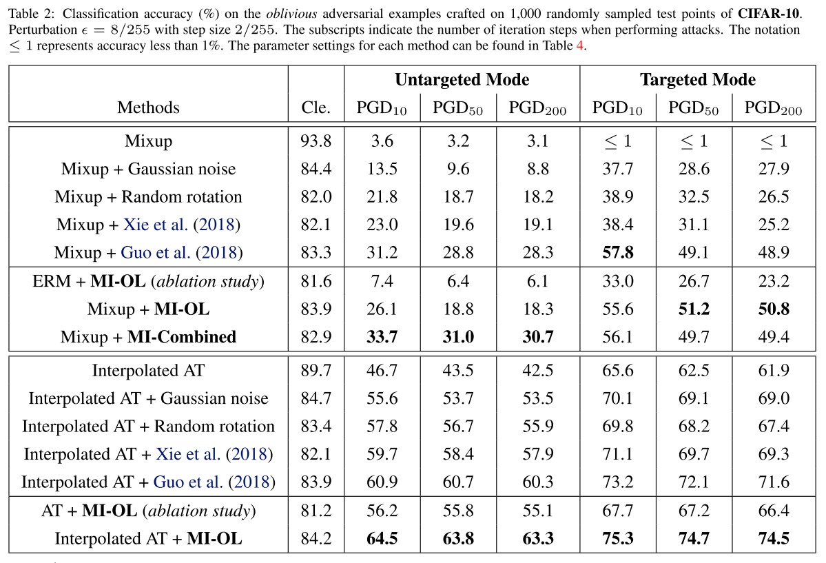
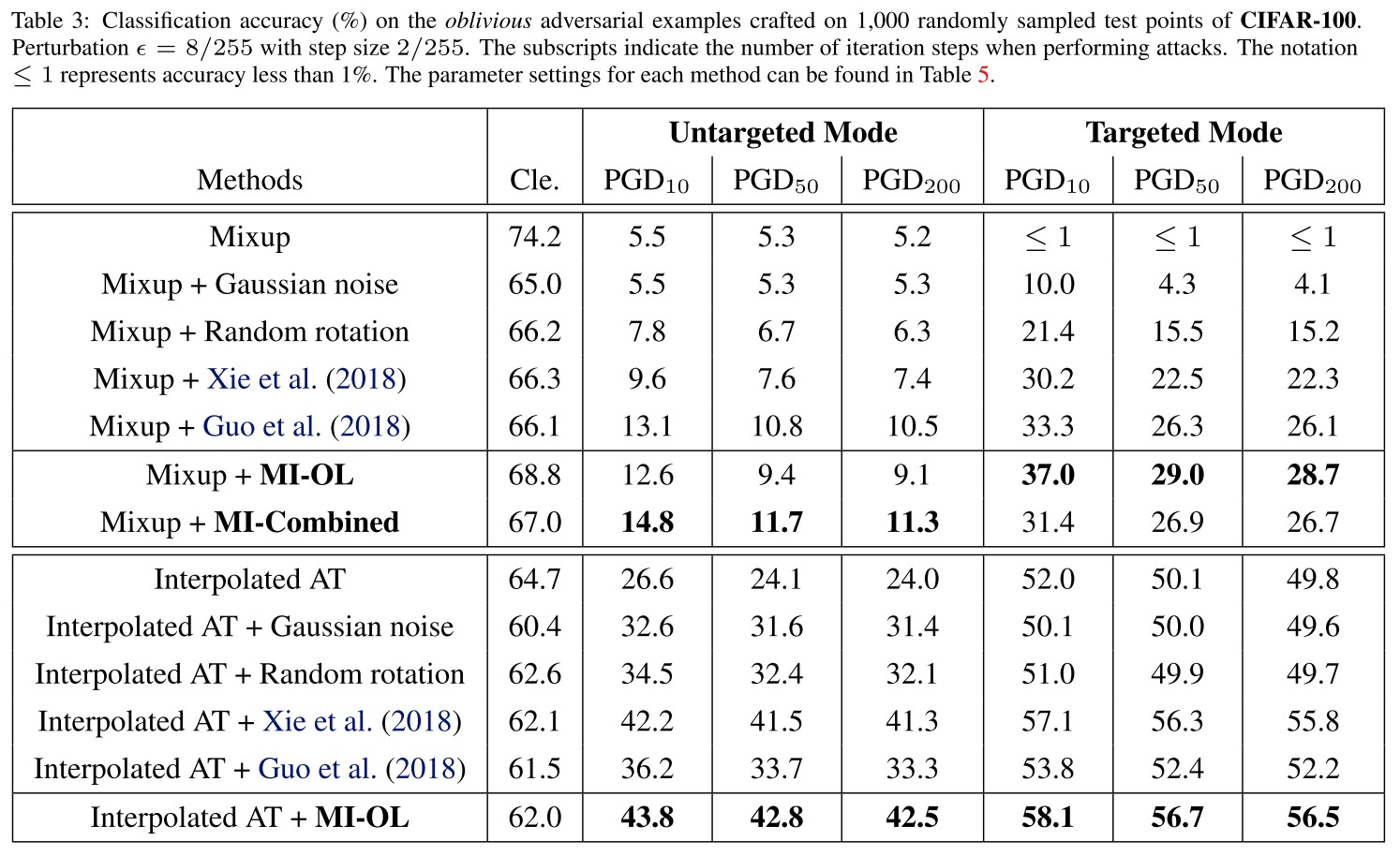
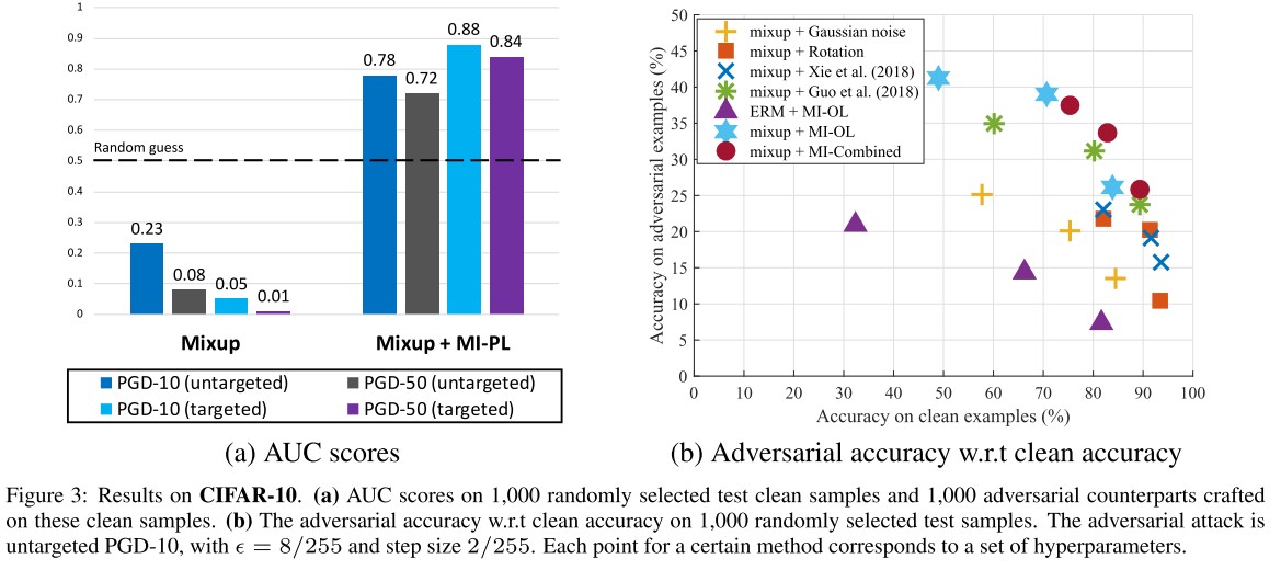
The results show that applying MI-PL in inference can better detect adversarial attacks, while directly detecting by the returned confidence without MI-PL performs even worse than a random guess.

As shown in these results, our MI method can significantly improve the robustness for the trained models with induced global linearity, and is compatible with training-phase defenses like the interpolated AT method.

It cannot work effectively independently.

They also evaluate on a customized adaptive attack.

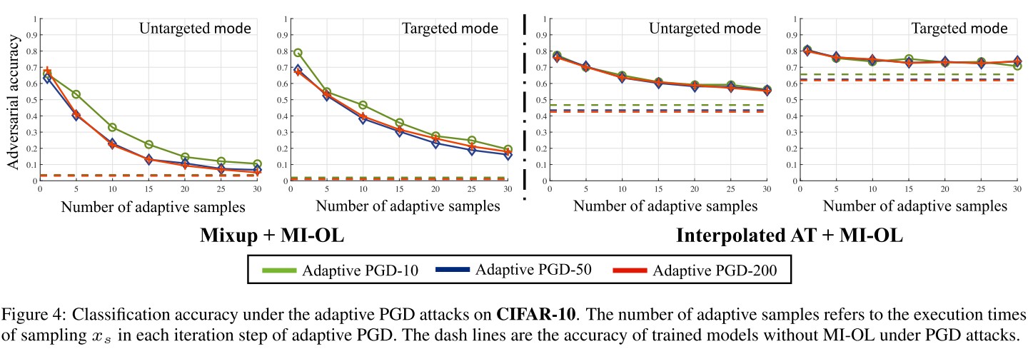
We can see that even under a strong adaptive attack, equipped with MI can still improve the robustness for the classification models.

Inspirations

This paper instantiates one of my ideas, and give a very comprehensive theoretical analysis. If the model follow the assumption that it works linearly on the combination of clean images, MI should work quite well, as demonstrated with Mixup Training and Interpolate AT.

The assumption is too strong, since most of the common classifiers do not function linearly between instances.

$x_s$ is very close to the clean image itself, the perturbation shrinkage will be very large, potentially fix the misclassification.