Adversarial Benchmark

By LI Haoyang 2020.11.10

Content

Benchmark datasets

ImageNet-C&ImageNet-P - ICLR 2019

Code: https://github.com/hendrycks/robustness

Dan Hendrycks, Thomas G. Dietterich. Benchmarking Neural Network Robustness to Common Corruptions and Surface Variations. ICLR 2019. arXiv:1807.01697

Our first benchmark, IMAGENET-C, standardizes and expands the corruption robustness topic, while showing which classifiers are preferable in safety-critical applications.

Then we propose a new dataset called IMAGENET-P which enables researchers to benchmark a classifier’s robustness to common perturbations

Corruptions and Perturbations

Consider the following objects:

$f:\mathcal{X}\to\mathcal{Y}$
$\mathcal{D}$
$C$
$\large{\varepsilon}$
$\Bbb{P}_C(c)$ $\Bbb{P}_{\large{\varepsilon}}(\varepsilon)$

$\mathcal{D}$ , i.e.

\Bbb{P}_{(x,y)\sim\mathcal{D}}(f(x)=y)

The corruption robustness of the classifier is

\Bbb{E}_{c\sim C}[\Bbb{P}_{(x,y)\sim\mathcal{D}}(f(c(x))=y)]

The adversarial robustness is a worst-case evaluation

\min_{||\delta||_p<b}\Bbb{P}_{(x,y)\sim\mathcal{D}}(f(x+\delta)=y)

The perturbation robustness is defined as

\Bbb{E}_{\varepsilon\sim\large{\varepsilon}}[\Bbb{P}_{(x,y)\sim\mathcal{D}}(f(\varepsilon(x))=f(x))]

which is an average evaluation.

$C$ $\large{\varepsilon}$ .

Common Corruptions

The corruptions they use include:

Gaussian noise
This corruption can appear in low-lighting conditions.
Shot noise (Poisson noise)
It is electronic noise caused by the discrete nature of light itself.
Impulse noise
It is a color analogue of salt-and-pepper noise and can be caused by bit errors.
Defocus blur
It occurs when an image is out of focus.
Frosted Glass Blur
It appears with “frosted glass” windows or panels.
Motion blur
It appears when a camera is moving quickly.
Zoom blur
It occurs when a camera moves toward an object rapidly.
Snow
It is a visually obstructive form of precipitation.
Frost
It forms when lenses or windows are coated with ice crystals.
Fog
It shrouds objects and is rendered with the diamond-square algorithm.
Brightness
It varies with daylight intensity.
Contrast
It can be high or low depending on lighting conditions and the photographed object’s color.
Elastic
This transformations stretch or contract small image regions.
Pixelation
It occurs when upsampling a lowresolution image.
JPEG
It is a lossy image compression format which introduces compression artifacts.

So many noises.

ImageNet-C

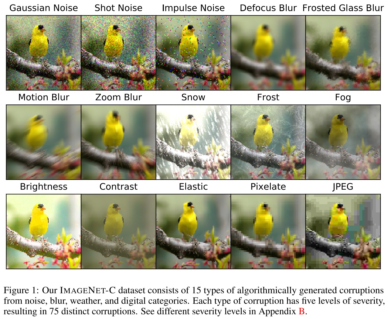
The IMAGENET-C benchmark consists of 15 diverse corruption types applied to validation images of ImageNet.

The corruptions are drawn from four main categories— noise, blur, weather, and digital—as shown in Figure 1.

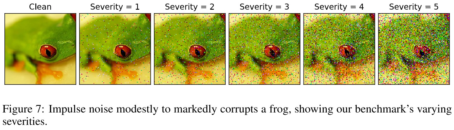
Each corruption type has five levels of severity since corruptions can manifest themselves at varying intensities.

Our benchmark tests networks with IMAGENET-C images, but networks should not be trained on these images.

Metrics

For each corruption, first compute the Corruption Error over 5 severities standardized by that of AlexNet, i.e.

\text{CE}_c^f=\left(\sum_{s=1}^5 E_{s,c}^f\right)\large{/}\left(\sum_{s=1}^5 E_{s,c}^{AlexNet}\right)

And the mCE is then computed as the average of the 15 Corruptions Error values corresponding to 15 types of corruptions.

The Relative mCE is the average of the following over 15 corruptions:

\text{CE}_c^f=\left(\sum_{s=1}^5 E_{s,c}^f-E_{clean}^f\right)\large{/}\left(\sum_{s=1}^5 E_{s,c}^{AlexNet}-E_{clean}^{AlexNet}\right)

This measures the relative robustness or the performance degradation when encountering corruptions.

ImageNet-P

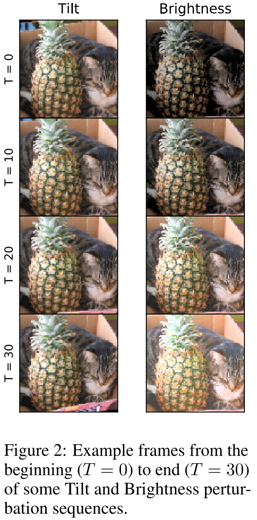
IMAGENET-P departs from IMAGENET-C by having perturbation sequences generated from each ImageNet validation image.

Each sequence contains more than 30 frames, so we counteract an increase in dataset size and evaluation time by using only 10 common perturbations.

However the remaining perturbation sequences have temporality, so that each frame of the sequence is a perturbation of the previous frame.

The perturbation sequences with temporality are created with motion blur, zoom blur, snow, brightness, translate, rotate, tilt (viewpoint variation through minor 3D rotations), and scale perturbations.

Metrics

$m$ perturbation sequences,i.e.

\mathcal{S}=\{(x_1^{(i)},x_2^{(i)},\dots,x_n^{(i)})\}_{i=1}^m

$n$ $i$ th perturbation.

Flip Probability $f:\mathcal{X}\to\{1,2,\dots,1000\}$ $\mathcal{S}$ $p$ is

\text{FP}_p^f=\frac{1}{m(n-1)}\sum_{i=1}^m\sum_{j=2}^n\bold{1}(f(x_j^{(i)})\neq f(x_{j-1}^{(i)})=\Bbb{P}_{x\sim\mathcal{S}}(f(x_j)\neq f(x_{j-1}))

$x_1^{(i)}$ is clean, the FP formula for noise sequences is

\text{FP}_p^f=\frac{1}{m(n-1)}\sum_{i=1}^m\sum_{j=2}^n\bold{1}(f(x_j^{(i)})\neq f(x_{1}^{(i)})=\Bbb{P}_{x\sim\mathcal{S}}(f(x_j)\neq f(x_{1})|j>1)

This metric calculates how many perturbed examples are classified correctly.

The Flip Rate is than defined as the standardized FP, i.e.

\text{FR}_p^f=\frac{\text{FP}_p^f}{\text{FP}_p^{AlexNet}}

The mFR is then acquired by averaging the FR across all perturbations.

$f$ $x$ $\tau(x)\in S_{1000}$ .

They define

d(\tau(x),\tau(x^\prime))=\sum_{i=1}^5\sum_{j=\min\{i,\sigma(i)\}+1}^{\max\{i,\sigma(i)\}}\bold{1}(1\le j-1\le 5)

$\sigma=(\tau(x))^{-1}\tau(x^\prime)$ $\tau(x)$ $\tau(x^\prime)$ are identical.

The unstandardized Top-5 Distance is the sum of top-5 distances across the entire perturbation sequences, i.e.

\text{uT5D}_p^f=\frac{1}{m(n-1)}\sum_{i=1}^m\sum_{j=2}^n d(\tau(x_j),\tau(x_{j-1}))=\Bbb{P}_{x\sim\mathcal{S}}(d(\tau(x_j),\tau(x_{j-1})))

Similarly, for noise perturbation sequences,

\text{uT5D}_p^f=\Bbb{E}_{x\sim\mathcal{S}}[d(\tau(x_j),\tau(x_1))|j>1]

and the standardized Top-5 Distance:

\text{T5D}_p^f=\frac{\text{uT5D}_p^f}{\text{uT5D}_p^{AlexNet}}

The mT5D is then acquired by averaging the Top-5 Distance.

Experiments

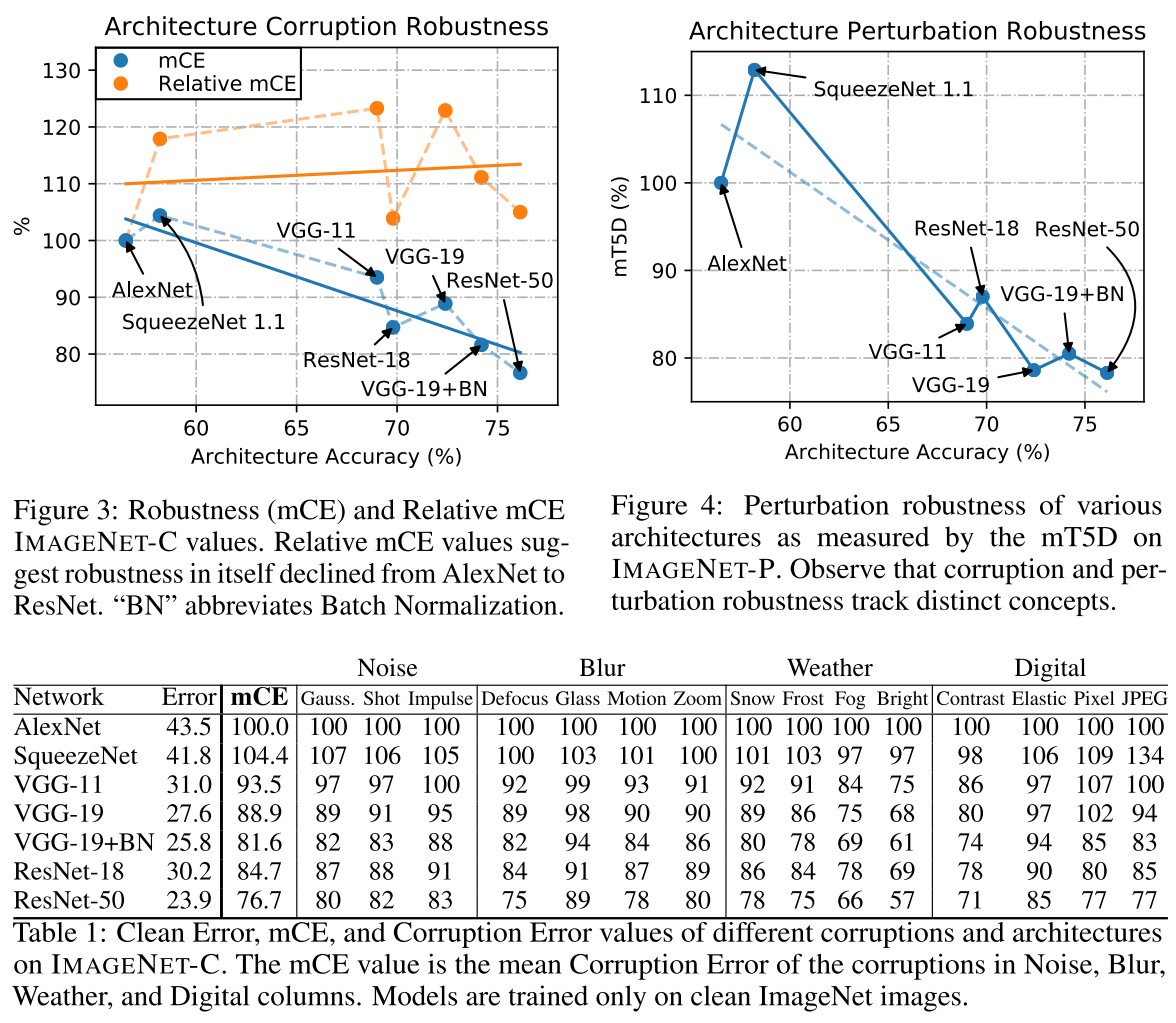
They test the robustness of different architectures, and discover that the recent architectures have better robustness, although it can be explained by the improvement of accuracy.

$\text{FP}_{Scale}^{ResNet-18} = 15.6\%$ $\text{uT5D}_{Scale}^{ResNet-18}$ is 3.6.

Clearly perturbations need not be adversarial to fool current classifiers.

They also study some robustness enhancement methods.

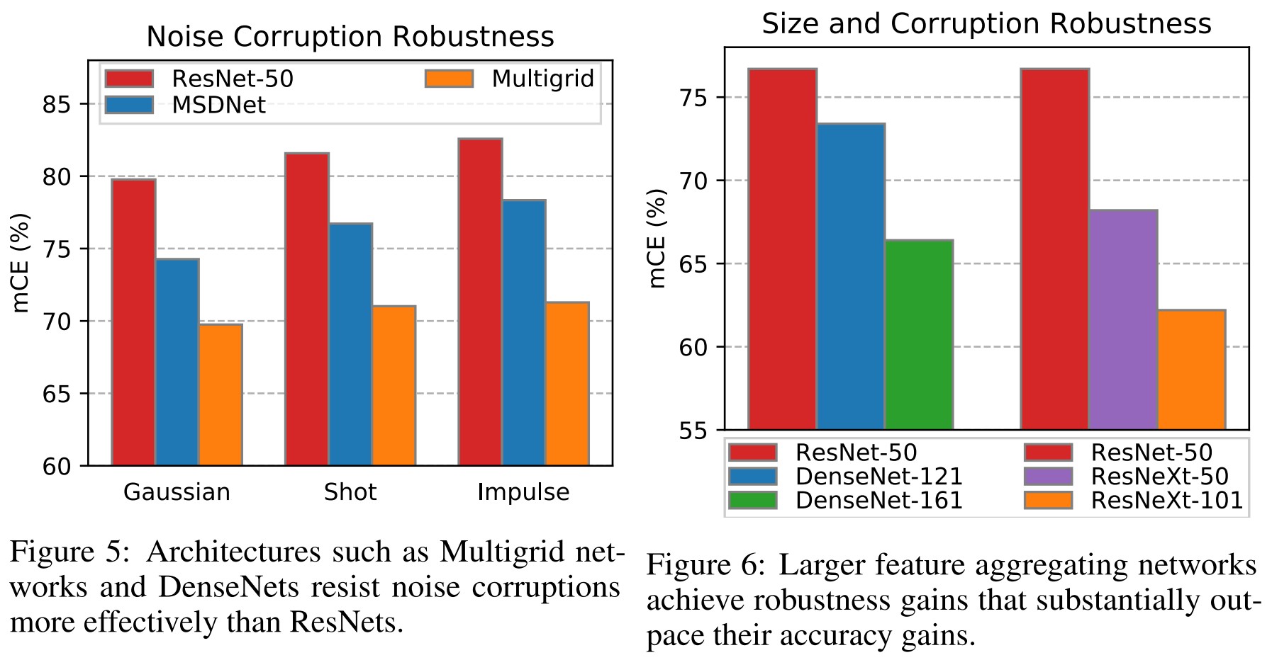
They discover that multiscale network, feature aggregation and larger network enhances the robustness.

Apparently more representations, more redundancy, and more capacity allow these massive models to operate more stably on corrupted inputs.

Training on Stylized ImageNet also helps.

When a ResNet-50 is trained on typical ImageNet images and stylized ImageNet images, the resulting model has an mCE of 69.3%, down from 76.7%.

And Adversarial Logit Pairing helps a lot.

ALP provides significant perturbation robustness even though it does not provide much adversarial perturbation robustness against all adversaries.

In point of fact, a publicly available Tiny ImageNet ResNet-50 model fine-tuned with ALP has a 41% and 40% relative decrease in the mFP and mT5D on TINY IMAGENET-P, respectively.

Inspirations

This is an ineteresting benchmark although the metrics are designed too complicated.

RobustBench - ICLR 2020

Leaderboard: https://robustbench.github.io/

Code: http://github.com/RobustBench/robustbench

Francesco Croce, Maksym Andriushchenko, Vikash Sehwag, Nicolas Flammarion, Mung Chiang, Prateek Mittal, Matthias Hein. RobustBench: a standardized adversarial robustness benchmark. ICLR 2020. arXiv:2010.09670

Our goal is to establish a standardized benchmark of adversarial robustness, which as accurately as possible reflects the robustness of the considered models within a reasonable computational budget.

They adopt the AutoAttack to benchmark SOTA classifiers, while ruling out the following methods:

Classifiers which have zero gradients with respect to the input (likely gradient masking)
Randomized classifiers (likely gradient masking)
Classifiers that contain an optimization loop in their predictions

Threat model

$f$ is assumed to be fully known to the attacker.

$l_p$ -perturbations, i.e.

\Delta_p=\{\bold{\delta}\in\R^d,||\delta||_p\le\varepsilon\}

$p=\infty$ .

The definition of successful adversarial perturbation they use is:

$\bold{x}\in\R^d$ $y\in\{1,\dots,C\}$ $f:\R^d\to\R^C$ successful adversarial perturbation $\Delta\sube\R^d$ $\bold{\delta}\in\R^d$ such that

\mathop{\arg\max}_{c\in\{1,\dots,C\}}f(\bold{x}+\bold{\delta})_c\neq y\text{ and }\bold{\delta}\in\Delta

$\Delta$ $\bold{x+\delta}$ $y$ as their true label.

robust accuracy $f$ $\Delta$ .

RobustBench

Features

A baseline worst-case evaluation with an ensemble of strong, standardized attacks which includes both white- and black-box attacks that can be optionally extended by adaptive evaluations
Clearly defined threat models that correspond to the ones used during training for submitted defenses
Evaluation of not only standard defenses, but also of more recent improvements.
The Model Zoo that provides convenient access to the most robust models from the literature which can be used for downstream tasks and facilitate the development of new standardized attacks

Restrictions

Only the classifier satisfying the following requirements are considered:

have in general non-zero gradients with respect to the inputs
have a fully deterministic forward pass
do not have an optimization loop in the forward pass

Initial setup

Adding new defenses

We require new entries to

satisfy the three restrictions formulated at the beginning of this section
to be accompanied by a publicly available paper (e.g., an arXiv preprint) describing the technique used to achieve the reported results
make checkpoints of the models available

The detailed instructions for adding new models can be found in our repository https://github.com/RobustBench/robustbench.

Analysis

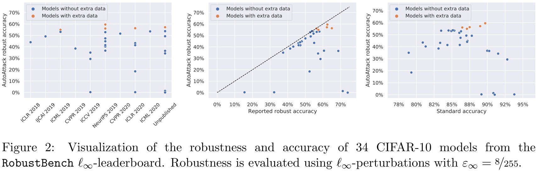
As shown in Figure 2

We observe that for multiple published defenses, the reported robust accuracy is highly overestimated
We also find that the use of extra data is able to alleviate the robustness-accuracy trade-off as suggested in previous work
$l_{\infty}$ -leaderboard (Carmon et al., 2019) is PGD adversarial training (Madry et al., 2018) enhanced only by using extra data (obtained via self-training with a standard classifier)

They test the performance of models across various distributional shift.

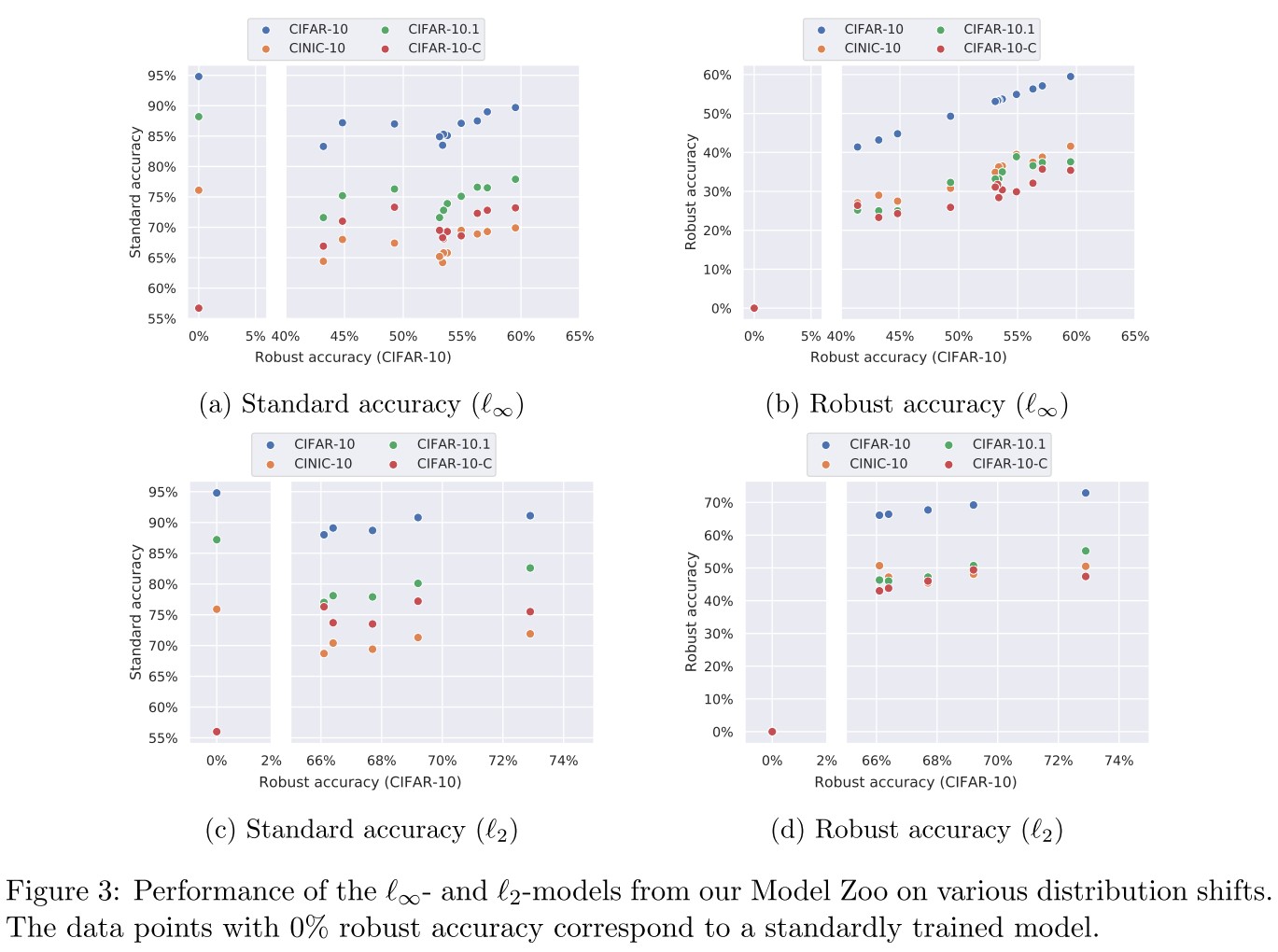
As shown in Figure 3

Robust networks have a similar trend in terms of the performance on these datasets as a standardly trained model
$l_2$ -norm) tend to give a significant improvement which agrees with the findings from the previous literature

And they also test the performance of out-of-distribution detection of models.

Ideally, a classifier should exhibit uncertainty in its predictions when evaluated on out-of-distribution (OOD) inputs.

In particular, Song et al. (2020) demonstrated that adversarial training (Madry et al., 2018) leads to degradation in the robustness against OOD data.

We use the area under the ROC curve (AUROC) to measure the success in the detection of OOD data.

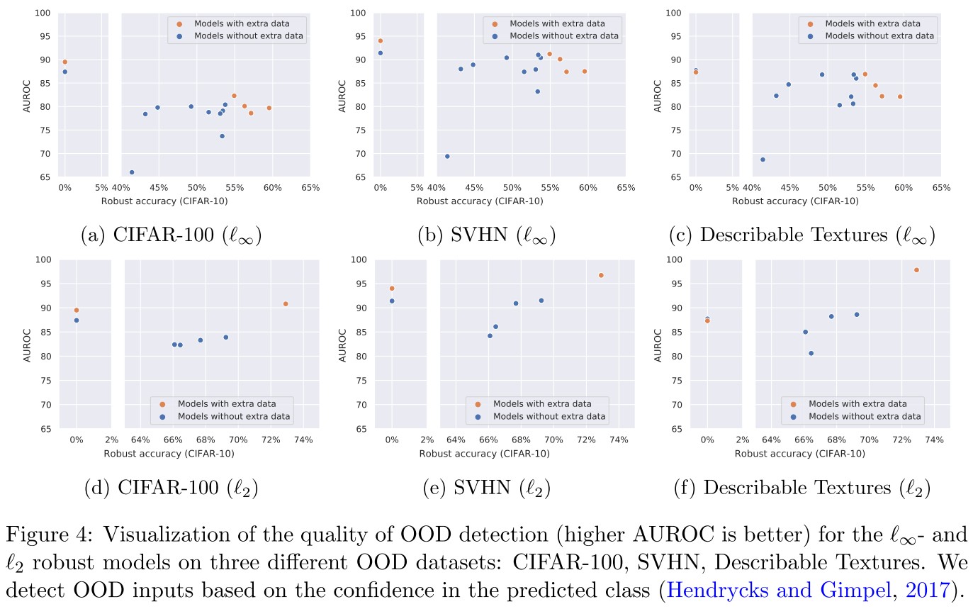
As shown in Figure 4

We find that compared to standard training, various robust training methods indeed lead to degradation of the OOD detection quality
With progress on robust accuracy, we find that robustness against OOD data plateaus and the use of extra data does not change this trend substantially.

This is expected, if adversarial examples and clean examples are from different distributions, then an adversarially robust model is expected to show worse performance in OOD detection quality.

Inspirations

This is a good benchmark.

ImageNet-A&ImageNet-O - 2020

Code: https://github.com/hendrycks/natural-adv-examples

Dan Hendrycks, Kevin Zhao, Steven Basart, Jacob Steinhardt, Dawn Song. Natural Adversarial Examples. arxiv preprint 2020. arXiv:1907.07174

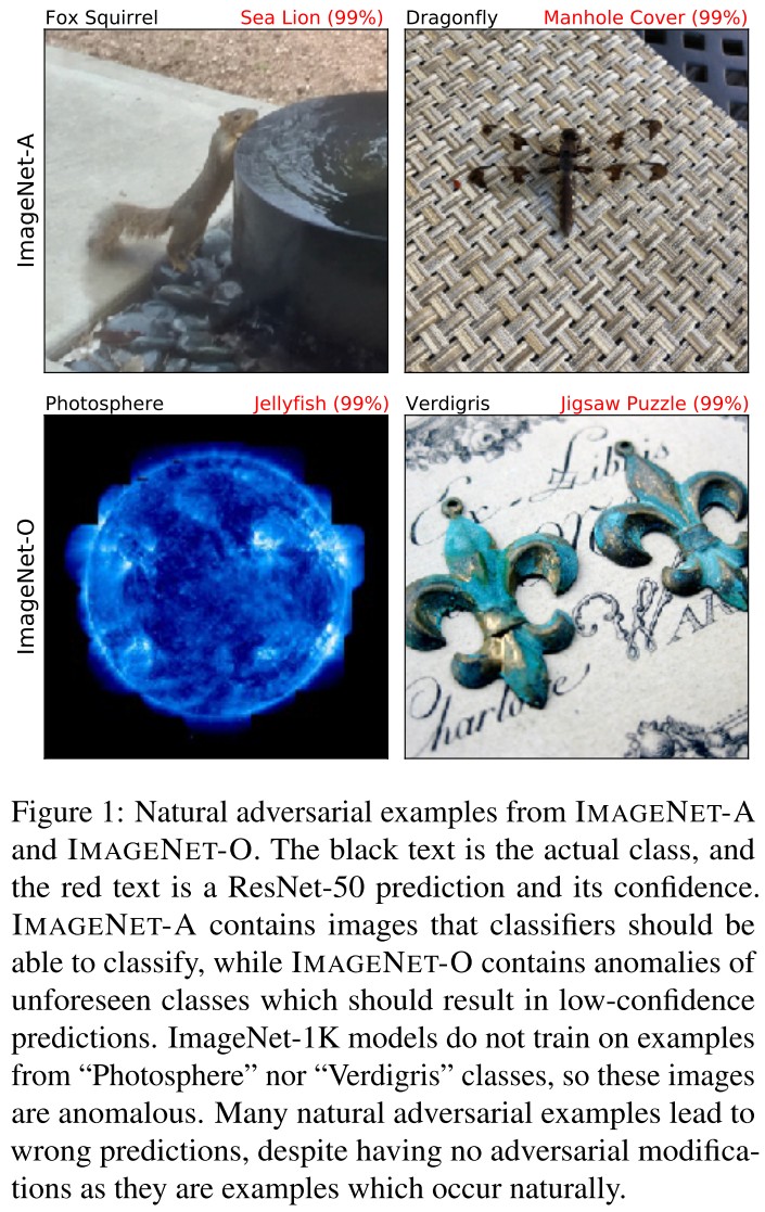
We introduce natural adversarial examples–real-world, unmodified, and naturally occurring examples that cause machine learning model performance to substantially degrade.

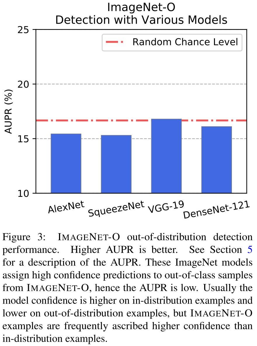
For example, on IMAGENET-A a DenseNet-121 obtains around 2% accuracy, an accuracy drop ofapproximately 90%, and its out-of-distribution detection performance on IMAGENET-O is near random chance levels.

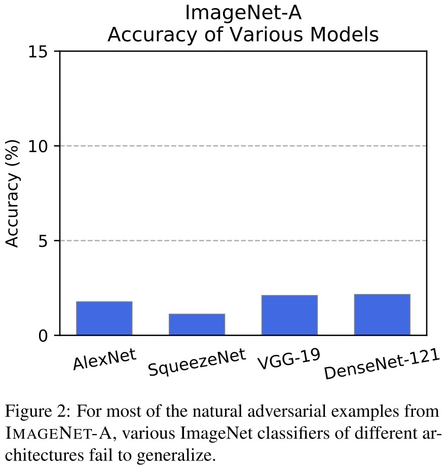
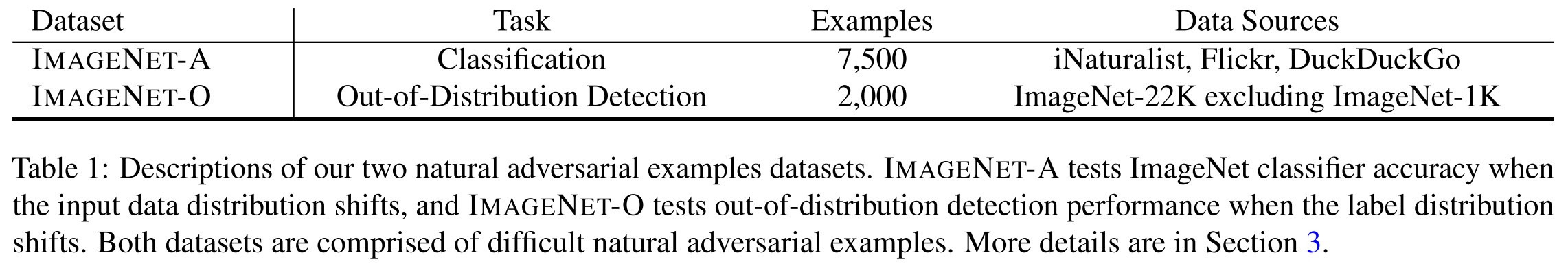
ImageNet-A

IMAGENET-A is a dataset of natural adversarial examples for ImageNet classifiers, or real-world examples that fool current classifiers

They first download numerous images related to an ImageNet class and delete the images that ResNet-50 classifiers correctly predict.

We select a 200-class subset of ImageNet-1K’s 1,000 classes so that errors among these 200 classes would be considered egregious.

They drop those classes that are two similar or old-fashioned.

ImageNet-O

Next, IMAGENET-O is a dataset of natural adversarial examples for ImageNet out-of-distribution detectors.

They download ImageNet-22K and delete examples from ImageNet-1K to create this dataset. For the remaining examples, they only keep examples that are classified by a ResNet-50 as an ImageNet-1K class with high confidence.

We again select a 200class subset of ImageNet-1K’s 1,000 classes. These 200 classes determine the in-distribution or the distribution that is considered usual.

Illustrative Classifier Failure Modes

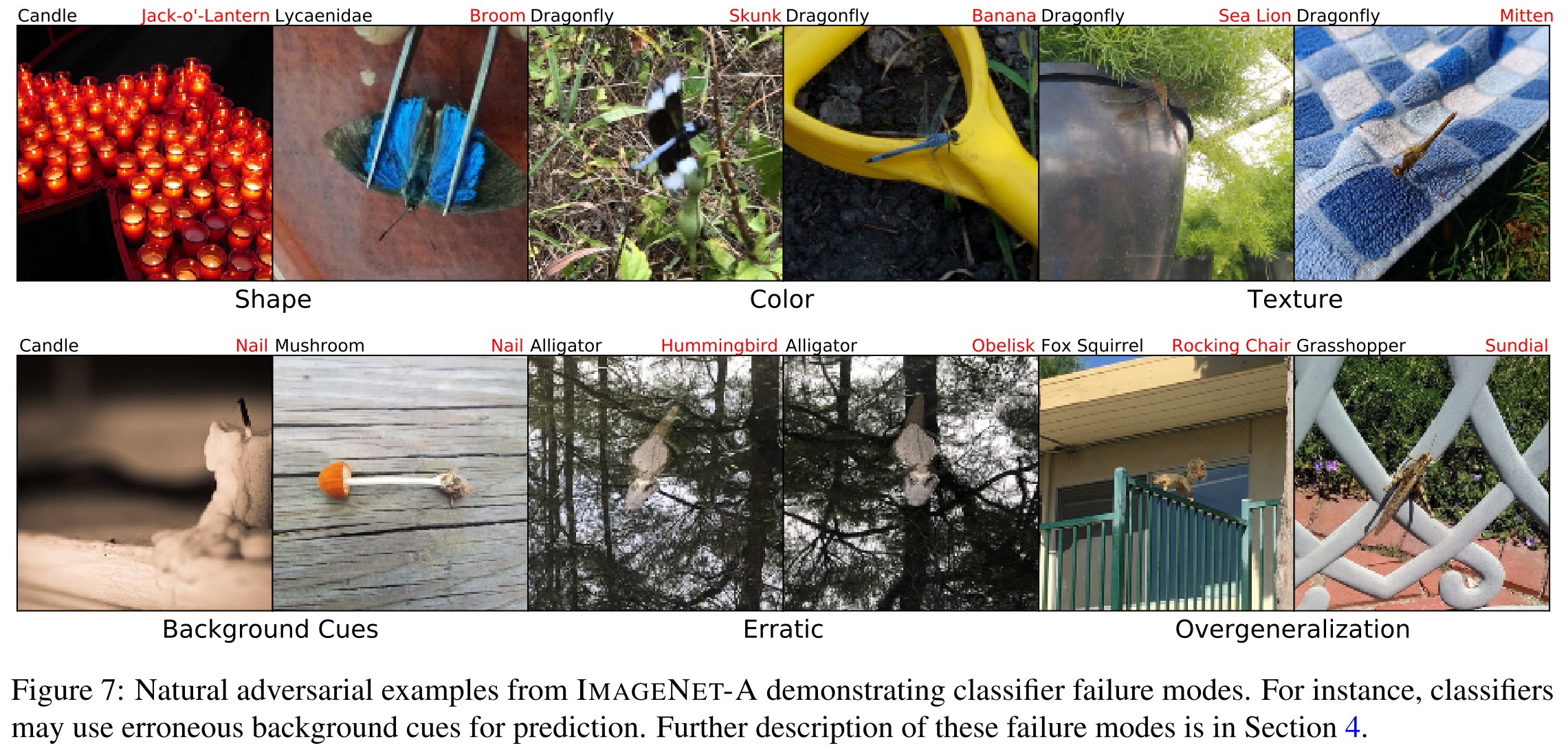
Classifiers may wrongly associate class with shape, color, texture or background, and they also demonstrate fickleness to small scene variations (e.g. the alligator in the down center of Figure 7, small variations induce different predictions).

Classifiers may also overgeneralize cues as demonstrated in the right down of Figure 7.

Experiments

Metrics

Our metric for assessing robustness to natural adversarial examples for classifiers is the top-1 accuracy on IMAGENET-A

Our metric for assessing out-of-distribution detection performance of NAEs is the area under the precision-recall curve (AUPR).

Data Augmentation

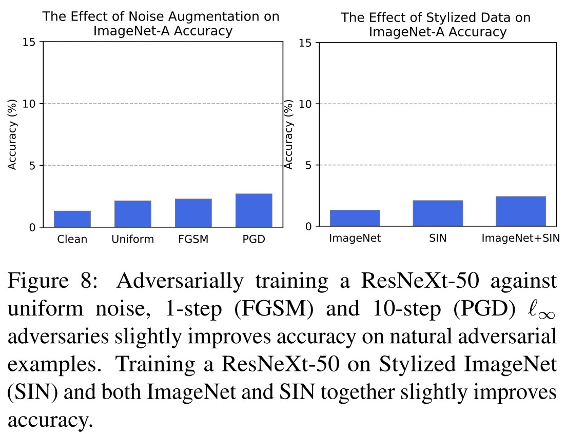
As shown in Figure 8, adversarial training hardly help and Reducing a ResNeXt-50’s texture bias by training with SIN (Stylized ImageNet) images does little to improve IMAGENET-A accuracy.

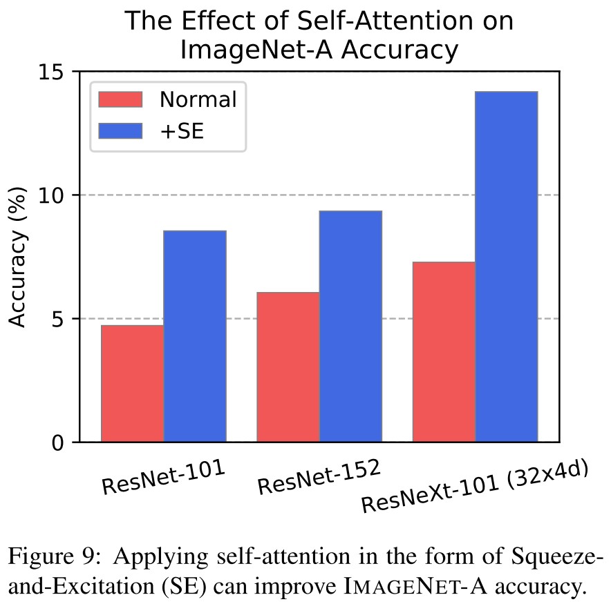
Architectural Changes Can Help

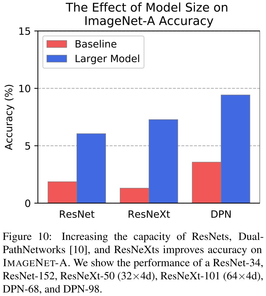
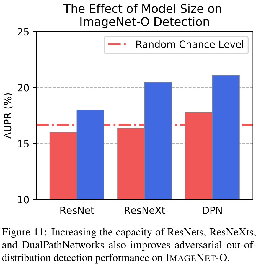
Inspirations

This dataset surely worth further exploration, but I think it's a little harsh on the classifier, especially as they set the metric as top-1 accuracy.

Benchmark attacks

AutoAttack- ICML 2020

Code: https://github.com/fra31/auto-attack

Francesco Croce, Matthias Hein. Reliable evaluation of adversarial robustness with an ensemble of diverse parameter-free attacks. ICML 2020. arXiv:2003.01690

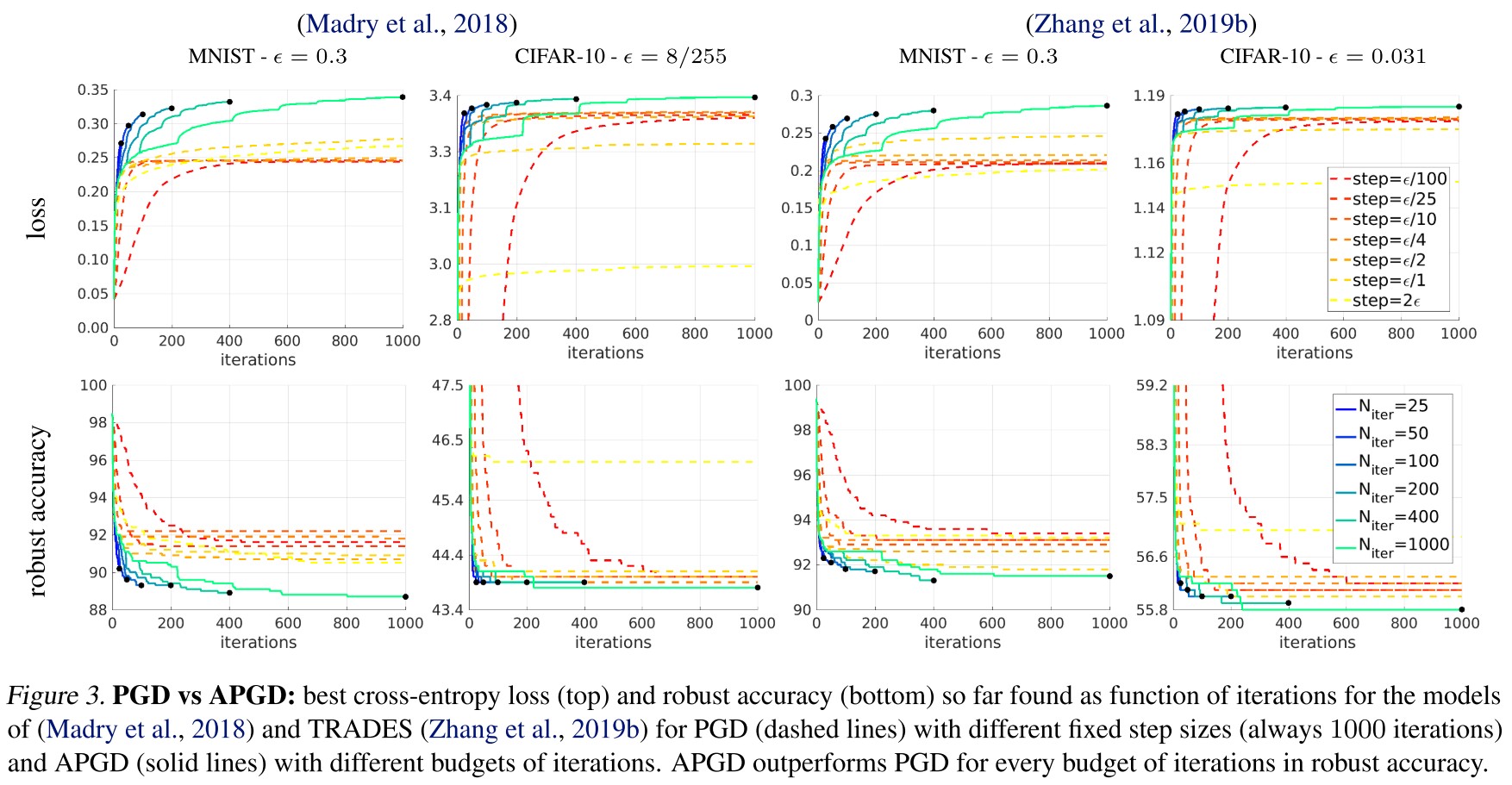
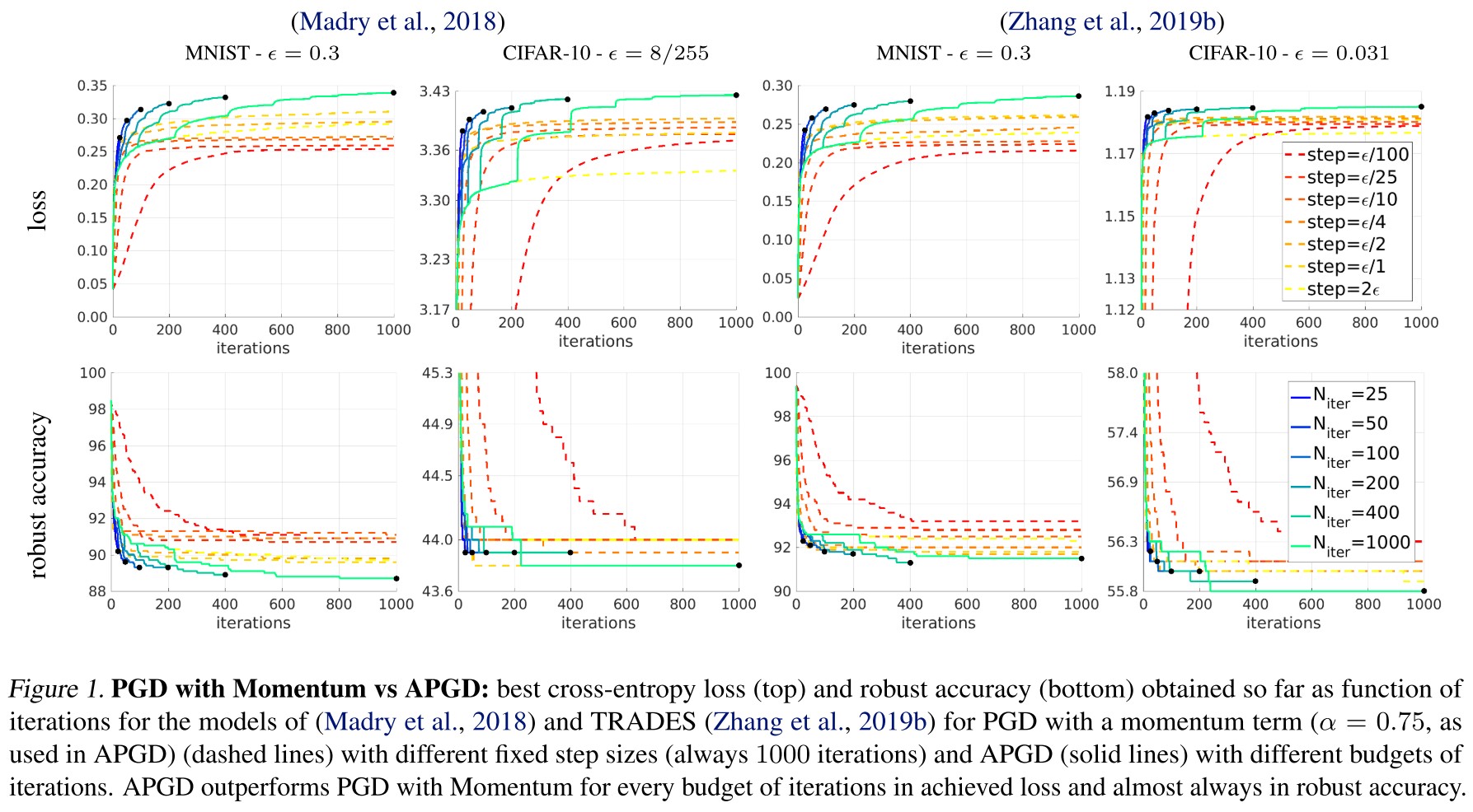
In this paper we first propose two extensions of the PGD-attack overcoming failures due to suboptimal step size and problems of the objective function.

The evaluation of proposed defenses is incomplete, hence leading a wrong impression of robustness. They modify the PGD attack to be parameter-free and propose to use it for evaluation.

They identify the fixed step size and the widely used cross-entropy loss as two major reasons for the failures of PGD and introduce more types of attacks to enrich the diversity, proposing a paremeter-free AutoAttack as an evaluation bench.

Adversarial example

The original mathematical forms are reformed here.

$K$ $g:\mathcal{D}\sube\R^k\to\R^K$ taking decisions according to

\mathop{\arg\max}_{k=1,\dots,K}g_k(x_{orig}),x_{orig}\in\R^k

$x_{orig}$ $c$ $g$ .

$d(\cdot,\cdot)$ $\epsilon>0$ , the threat model (attack space) is defined as

\mathcal{S}:=\{z\in\mathcal{D}|d(x_{orig},z)\le \epsilon\}

$l_p$ -norm, i.e.

d(x,z):=||z-x||_p,\mathcal{D}\in[0,1]^d

$z$ $g$ $x_{orig}$ w.r.t the threat model if

\mathop{\arg\max}_{k=1,\dots,K}g_k(z)\neq c,z\in\mathcal{S}

$z$ $L$ and solve the constrained optimization problem

\max_{z\in\mathcal{S}}L(g(z),c)

Projected Gradient Descent (PGD) $k$ th step as

x^{(k+1)}=P_{\mathcal{S}}(x^{(k)}+\eta^{(k)}\nabla f(x^{(k)}))

$f:\R^d\to\R$ $P_{\mathcal{S}}:\R^k\to\mathcal{S}$ projects the perturbed data point back to the attack space.

$\eta^{(k)}=\eta$ $x_{orig}$ $x_{orig}+\zeta$ , i.e. a random start point in the attack space.

Auto-PGD

They claim three drawbacks of initial PGD:

Suboptimal fixed step size
Budget agnostic overall scheme
Unaware of the trend (i.e. agnostic of the current situation of the optimization process)

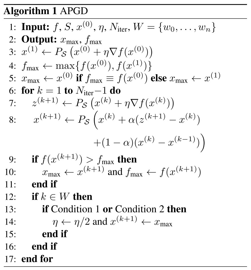
They propose to add a momentum term for the update:

x^{(k+1)}=P_{\mathcal{S}}(x^{(k)}+\alpha\cdot(z^{(k+1)}-x^{(k)})\\ +(1-\alpha)\cdot(x^{(k)}-x^{(k-1)})),\alpha\in[0,1]

And add two conditions to decide when to restore the recorded best point and decay the step size:

$\sum_{i=w_{j-1}}^{w_j-1}\bold{1}_{f(x^{(i+1)})>f(x^{(i)})}<\rho\cdot(w_j-w_{j-1})$
$\eta^{(w_j-1)}\equiv \eta^{(w_j)}$ $f_{max}^{(w_j-1)}\equiv f_{max}^{(w_j)}$

Condition 1 $w_{j-1}$ $f$ . If this holds for a fraction of total update steps since last checkpoints, then the step size is considered properly to be kept and the condition will be false.

Condition 2 holds true if without step size adjustment, the objective is not increased since last checkpoint.

If one of the conditions above hold true, the data point is restarted at the best one with the step size halved, i.e.

\eta\gets\eta/2,x^{(k+1)}\gets x_{max}

$N_{iter}$ .

Alternative loss function

The widely used cross-entropy loss is affected by the scale of logits, i.e. small logits cause gradient vanishing (due to the finite arithmetic).

$\alpha\in\{1,10^1,10^2,10^3\}$ .

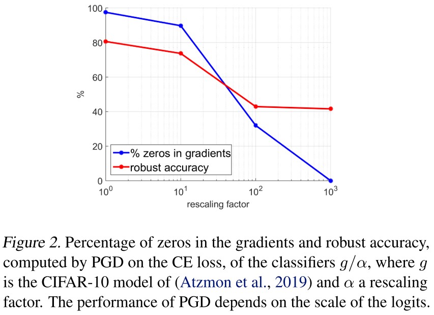
As shown in Figure 2, without rescaling the gradient vanishes almost for every coordinate, which leads to a relatively overestimated robust accuracy.

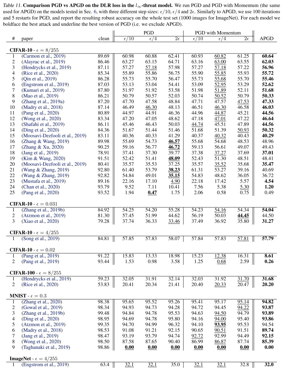
They propose the Difference of Logits Ratio (DLR) loss, designed to be both shift and rescaling invariant, i.e.

\text{DLR}(x,y)=-\frac{z_y-\max_{i\neq y}z_i}{z_{\pi_1}-z_{\pi_3}}

$\pi$ $z$ in decreasing order.

For a classifier, minimizing DLR means to maximize the difference between the correct logit and the second largest logit while keeping the difference to be proportional to be difference of the largest logit and the thrid largest logit.

For adversary, the process is reversed.

And a targeted version

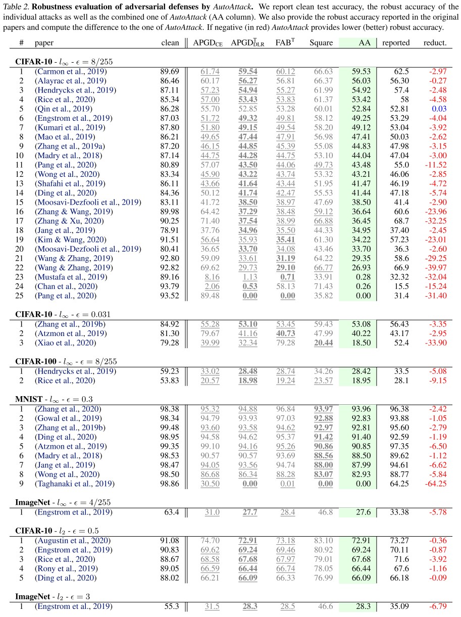
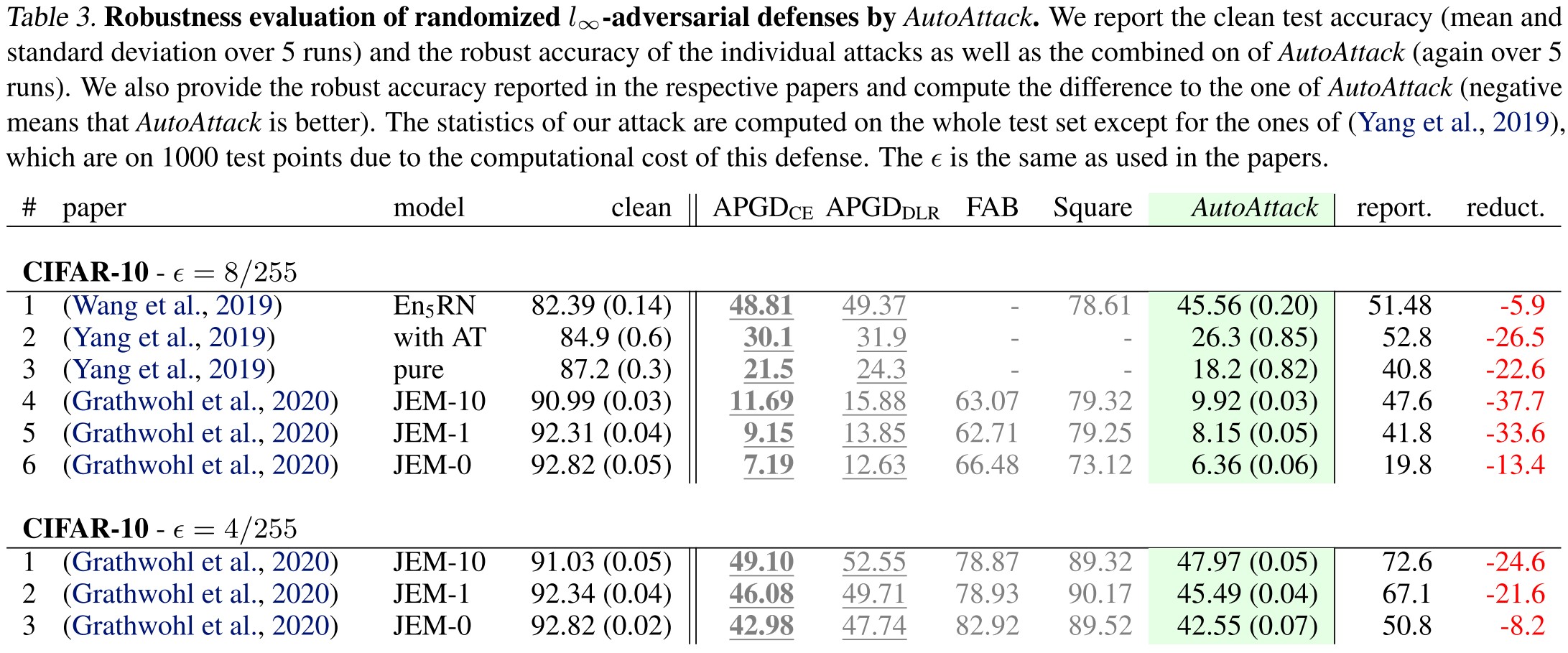
\text{Targeted-DLR}(x,y)=-\frac{z_y-z_t}{z_{\pi_1}-(z_{\pi_3}+z_{\pi_4})/2}

AutoAttack

We combine our two parameter-free versions of PGD, APGD_CE and APGD_DLR, with two existing complementary attacks, FAB (Croce & Hein, 2020) and Square Attack (Andriushchenko et al., 2020), to form the ensemble AutoAttack.

Inspirations

It seems that using unlabeled data is the best approach in CIFAR-10, which leads to the problem of robustness to the direction of data augmentation.